Note: 10x Genomics does not provide support for community-developed tools and makes no guarantees regarding their function or performance. Please contact tool developers with any questions. If you have feedback about Analysis Guides, please email analysis-guides@10xgenomics.com.
Clustering and classification are fundamental computational techniques used to identify groups of cells that share similar characteristics, often based on their gene expression profiles. This process helps us uncover the hidden biological stories within a dataset, from identifying rare cell types to characterizing the overall heterogeneity of a cell population.
Standard single cell RNA sequencing (scRNA-seq) datasets, generated with 10x Genomics Chromium assays, rely primarily on gene expression features from individual cells. By contrast, the field of spatial transcriptomics encompasses technologies such as 10x Genomics Visium HD and Xenium In Situ, which capture gene expression along with the spatial context, but differ in their resolution and molecular profiling approaches. Visium HD provides spatially resolved transcriptomic data at 2-µm resolution across tissue sections. Increasingly, downstream clustering for Visium HD is performed on cell-segmented expression profiles, rather than raw bins, to better align results with biological cells. In contrast, Xenium In Situ enables high-resolution, subcellular mapping of gene expression at the single-molecule level directly within tissue sections. These technologies have contributed to a growing number of methods that integrate spatial information into the clustering process.
This article focuses on clustering and classification methods for Chromium, Visium, and Xenium datasets. We first review established techniques for analyzing single cell data, then focus on spatially-informed clustering approaches tailored for the variable resolutions of Visium data (from spots to HD squares) and Xenium data (high-resolution cellular and subcellular). Many methods originally developed for Visium data may potentially be adapted to Xenium data, given its enriched spatial and gene expression information, thus expanding the toolbox available for integrative analysis.
The table below summarizes typical analysis questions for single cell and spatial datasets, the recommended clustering or classification strategies, and the key input sources required. This may help inform decisions on when a single cell analysis is sufficient and when spatially-informed methods add value.
| Data Type | Typical Biological Question | Recommended Clustering Strategy |
|---|---|---|
| Chromium (scRNA-seq) | Identify major and rare cell types; build a cell-type atlas across samples | Standard graph-based clustering (with optimal sub-clustering for rare populations); occasional supervised classifiers for annotation |
| Visium (tissue-level domains) | Define broad tissue regions (e.g., tumor vs. stroma, cortical layers, fibrotic vs. normal) | Neighborhood-aware or morphology-integrated spatial clustering; focus on spatial smoothness and domain boundaries |
| Visium (fine-grained patterns within mixed spots) | Resolve finer spatial structure where each spot contains multiple cell types (e.g., layered retina, tumor-immune interface) | Resolution-enhancing spatial clustering to computationally subdivide spots |
| Visium HD (cell-segmented) | Resolve fine-scale tissue architecture and cell states where reliable cell segmentation is available, enabling more biologically interpretable clustering than bin-based representations. | Cell-level clustering on segmented expression profiles; apply standard graph-based or neighborhood-aware clustering to segmented cells to achieve cleaner, more interpretable clusters than bin-based approaches; fallback to spatial clustering on fixed-resolution bins when segmentation is not available. |
| Xenium (cell types in situ) | Identify cell types and states directly in tissue, at single cell resolution | Standard single cell clustering approaches can be applied to segmented cells, optionally augmented with local neighborhood information |
| Xenium (microenvironments and niches) | Define cell-cell interaction zones (e.g., immune niches, tumor borders, stem-cell niches) | Neighborhood-aware spatial clustering where the local environment is explicitly modeled. |
| Single cell and spatial (cross-modality integration) | Transfer single cell-defined cell types onto spatial data; map cell states into tissue context | 2-step workflow: a) single cell graph-based clustering b) label transfer, deconvolution and spatial clustering. |
When analyzing single cell and spatial data, the choice of clustering approach depends on the biological question, and the nature of the research project. Broadly, clustering and classification algorithms for these types of datasets fall into two categories:
- Unsupervised clustering identifies patterns without prior information. These clustering approaches are used to identify novel cell populations and intrinsic structure in the data without prior assumptions. They are useful for discovery and hypothesis generation. For example, graph-based methods can be used to uncover unbiased clusters in single cell data, or incorporate neighborhood information into spatial data.
- Supervised methods uses references to guide classification. These approaches are used to assign known identities based on training data, references, or marker sets. These methods are useful for annotation and reproducibility. Examples include label transfer from reference datasets for Xenium In Situ data.
| Approach | Example Methods | When to Use | Notes |
|---|---|---|---|
| Unsupervised | Graph-based (Leiden, Louvain), K-means, Hierarchical, Hidden Markov Models, Deep Learning | Discover new/rare populations | Flexible, parameter-sensitive |
| Supervised | Support Vector Machines (SVMs), Decision Trees, Label Transfer | Assign known cell types | Relies on curated reference data |
The following sections will highlight commonly-used algorithms under these two approaches for single cell and spatial datasets.
The following clustering methods are foundational to single cell analysis, where the primary goal is to organize dissociated cells into meaningful groups based on their gene expression profiles. While these techniques are also useful for spatial analysis, their principles are best introduced in the context of single cell data. Below is a summary of these core methods along with their key features and common use cases:
| Method | Approach | Key Features | Use Case |
|---|---|---|---|
| Graph-based | Unsupervised | Scales to 100k+ cells; can capture complex relationships between individual cells; resolution tuning | Standard for large datasets; widely adopted in the community (e.g., Seurat, Scanpy) |
| K-means | Unsupervised | Requires k upfront | Coarse clustering, broad groups |
| Hierarchical | Unsupervised | Builds cluster trees (dendrograms) | Small datasets, visualization (cell lineages) |
| SVMs/Decision Trees | Supervised | Leverages references for classification | Cell annotation (for well-defined tissue/cell types) |
A common strategy for analyzing single cell data is to first perform a coarse clustering to identify major cell types, followed by re-clustering within individual clusters to capture finer subtypes and heterogeneity. This approach is particularly useful for large or diverse cell populations, as it helps distinguish broad cell types before refining sub-populations. How exactly this is executed depends on the underlying mathematical framework of the chosen algorithm. The details of some prominent methods are listed below:
- Graph-based unsupervised clustering involves building a sparse nearest-neighbor graph to identify highly-connected "modules" or "clusters". A major advantage of this method is its scalability, driven by efficient use of a sparse nearest-neighbor graph allowing for superior memory and computational efficiency. This is crucial in single cell analysis, where datasets can contain millions of cells. As these datasets grow, efficient methods are needed to handle them without excessive computational time or memory usage, making scalability a key benefit. However, the sensitivity to parameter settings can impact the quality and interpretation of the resulting clusters, as illustrated in a study by Zheng et al. 2017, Cell.
- In K-means unsupervised clustering, a fundamental assumption is that we have a priori knowledge of the expected number of clusters within the dataset, and the algorithm assigns cells according to this predetermined number. The "k" value represents the number of clusters. It is typically chosen based on prior knowledge, exploratory analysis (e.g., elbow plots), or domain expertise, rather than being fixed by the algorithm itself. This approach is particularly useful for large or diverse cell populations to help distinguish broad cell types before refining subpopulations. One example is highlighted in this study, Identifying cell populations with scRNASeq, where k-means clustering was used to identify cell subpopulations in large datasets from tissues including the mouse hypothalamus.
- Hierarchical unsupervised clustering is a method that builds distances between data points through a series of successive fusions of individual objects, thus building a hierarchy by combining the nearest data points and merging them into clusters. This offers flexibility and a visual representation in understanding relationships among data points. However, this analysis can be computationally intensive when dealing with large datasets. In this study, this method was used to analyze early organ development in human embryos, offering valuable insights into cellular organization and developmental processes.
- Decision trees are supervised machine learning algorithms used in scRNA-seq to classify cells based on gene expression profiles. They work by recursively splitting the data at decision nodes to create distinct classes, making them useful for cell typing and subtype identification. Decision trees are straightforward to interpret, as they provide clear rules for classifying cells. However, the method can struggle with high-dimensional data and may overfit, especially when the number of features exceeds the number of samples. Pruning and setting depth limits can help mitigate overfitting. Despite these challenges, decision trees are effective for classification tasks and can provide insights into the most important features driving cell-type differentiation and gene expression patterns.
Below are some third party tools and clustering methods that are commonly used in the single cell community.
| Tools | primarily uses prior knowledge | Clustering Process | Tutorial | Use-cases | References |
|---|---|---|---|---|---|
| CellAssign (R) | Yes | Guided clustering | Automated, probabilistic assignment of scRNA-seq to cell types | Assign specific cell types using a known marker gene list (Tumor Microenvironemnt) | Zhang et al., Nature Methods, 2019 |
| CIDR (R) | No | Modified K-means clustering (K-PCA) | Clustering through Imputation and Dimensionality Reduction | Datasets with high dropout dates; clustering without heavy imputation steps | Lin et al., Genome Biology, 2017 |
| CytoTRACE (python) | Yes | Decision tree and Hierarchical clustering | Cellular (Cyto) Trajectory Reconstruction Analysis using gene Counts and Expression | Predicting differentiation states; identifying stem-like vs differentiated cells. | Gulati et al., Science, 2020 |
| Monocle (R) | No | Leiden clustering | Clustering and classifying your cells | Trajectory inference; ordering cells along a developmental timeline | Trapnell et al., Nature Biotechnology, 2014 |
| RCA (R) | Yes | Correlation score between reference and the single cell data, in supervised manner. | Reference Component Analysis | Reference-based annotation; ensuring consistency with a specific reference atlas | Li et al., Nature Genetics, 2017 |
| SC3 (R) | No | Hierarchical clustering | SC3 package manual | High-accuracy consensus clustering; best for smaller, high-quality datasets (conputationally intensive) | Kiselev et al., Nature Methods, 2017 |
| Scanpy (Python) | No | Multiple clustering options: Louvain, leiden, K-means, Hierarchical etc | Preprocessing and clustering 3k PBMCs | Processing massive datasets (1M+ cells) efficiently; Python-based workflows | Wolf et al., Genome Biology, 2018 |
| scmap_cluster (R) | No | Hierarchical clustering | Scmap package vignette | Projecting cells onto a reference datasets for fast annotation | Vladimir et al., Nature Methods, 2018 |
| Azimuth (R/web) | Yes | Reference-based mapping; (Anchor transfer & WNN projection) | Azimuth tutorial | Seurat has standard, versatile pipeline for discovery, integration, and multimodal analysis; also include automated cell-type annotation using azimuth | Hao et al., Cell, 2021 |
| Seurat_clustering (R) | No | Graph-based (Louvain) & Leiden clustering | Seurat Clustering Tutorial | Seurat has standard, versatile pipeline for discovery, integration, and multimodal analysis; also include automated cell-type annotation using azimuth | Stuart et al., Cell, 2019 |
| SHARP (R) | No | Non-negative matrix factorization (NMF) and consensus clustering, scalable and very fast | Single-cell RNA-seq Hyper-fast and Accurate processing via ensemble Random Projection | Hyper-fast clustering for very large datasets | Shibiao et al., Genome Research, 2020 |
| SingleR (R) | Yes | Guided clustering | Assigning cell types with SingleR | Automated cell type annotation comparing query data to reference datasets | Aran et al., Nature Immunology, 2019 |
If the goal is to detect rare cell types, employing unsupervised methodologies akin to those found in Seurat or monocle3 is advantageous due to their flexibility in exploring data without prior assumptions. Conversely, for classification based on a pre-established reference, tools like RCA or CytoTRACE offer robust options for supervised analysis, ensuring consistency and reliability when comparing new data to known cell types.
Spatial transcriptomics provide a significant advantage over dissociated single cell techniques by preserving the native location of cells within a tissue, linking gene expression profiles to their spatial context. This allows spatial clustering algorithms to group cells, squares, or spots based not only on transcriptional similarity but also on their spatial relationships, revealing tissue architecture and multicellular organization.
Unlike traditional scRNA-seq clustering methods that operate on a gene expression matrix alone, spatial clustering algorithms leverage two primary inputs: the gene expression matrix and the spatial coordinates of each cell or measurement spot. Optionally, additional data modalities, such as H&E images or segmentation details, could be used. By integrating these inputs, spatial clustering algorithms can identify clusters that are both transcriptionally distinct and spatially coherent. Choosing the most appropriate algorithm therefore depends on the data quality, the biological question, the experimental goal of the study, and the available inputs.
The major spatial clustering tools can be conceptually grouped by the primary type of information they integrate alongside gene expression data.
| Methods | Key Input (Beyond Expression & Coordinates) | Example Tools | Use case |
|---|---|---|---|
| Neighborhood-aware | None | BANKSY | Defining functional domains where the local environment and cell-cell signaling are important (e.g., tumor-immune boundary). |
| Morphology Integration | H&E Histology Image | SpaGCN, stLearn | Aligning transcriptional domains with anatomically distinct features visible in the tissue slide (e.g., cortical layers in the brain). |
| Resolution Enhancement | None (uses statistical modeling) | BayesSpace | Computationally increasing the resolution of spot-based data to uncover fine-grained spatial patterns hidden by technical limits. |
BANKSY
- Publication: BANKSY: A Spatial Omics Algorithm that Unifies Cell Type Clustering and Tissue Domain Segmentation
- Source code: https://github.com/prabhakarlab/Banksy and https://github.com/prabhakarlab/Banksy_py (Python)
- Tutorial: BANKSY tutorial
- Algorithm: BANKSY operates on the principle that a cell's identity is defined by both its intrinsic gene expression and that of its surrounding neighborhood. It creates an "augmented" expression matrix that combines a cell's own profile with the aggregated profile of its neighbors. A key parameter, λ (lambda), allows the user to tune the influence of the neighborhood, enabling a flexible analysis that can prioritize either cell-intrinsic states or broader tissue environments.
- Use case: Use BANKSY when you want to identify tissue regions where the local cellular environment is a key defining feature. For example, in a tumor microenvironment, you could use it to find "hotspots" of immune cell activity that influence nearby cancer cells. Or in developmental biology, to identify organizing centers where a small group of cells patterns the development of its neighbors. The tunable λ parameter controls how much influence a cell's neighborhood has on its clustering; lower values emphasize individual cell identity, while higher values highlight spatial context. In practice, λ is typically chosen empirically by testing a small range (e.g., 0–1) and selecting the value that yields biologically meaningful clusters or consistent domain patterns. BANKSY is actively recommended and used for Visium (including cell-segmented Visium HD) for neighborhood-aware clustering. It is also the recommended choice for very large datasets because it scales efficiently to millions of cells without requiring specialized hardware.
SpaGCN
- Publication: SpaGCN: Integrating gene expression, spatial location and histology to identify spatial domains and spatially variable genes by graph convolutional network
- Source code: https://github.com/jianhuupenn/SpaGCN
- Tutorial: SpaGCN tutorial
- Algorithm: SpaGCN integrates three sources of data: gene expression, spatial coordinates, and histology from the H&E image. It constructs a graph where spots are connected based on their spatial proximity and histological similarity. A graph convolutional network is then used to aggregate gene expression information from neighboring spots, effectively smoothing the data in a way that respects the underlying tissue morphology.
- Use case: SpaGCN is the ideal tool when you expect the transcriptional domains in your tissue to align closely with structures visible in the histology slide. For instance, if you are analyzing a brain slice with distinct cortical layers, or a kidney section with clearly defined glomeruli and tubules, SpaGCN can delineate these structures with high fidelity by ensuring that cluster boundaries respect both the molecular and the morphological data. For massive datasets (Xenium, binned Visium HD), utilizing GPU is recommended to maintain reasonable runtimes during the graph construction phase.
stLearn
- Publication: stLearn: integrating spatial location, tissue morphology and gene expression to find cell types, cell-cell interactions and spatial trajectories within undissociated tissues
- Tutorial: stSME clustering tutorial
- Algorithm: stLearn also integrates H&E image features with gene expression, but through a different mechanism. It first processes the image to extract morphological features for each spot. It then normalizes each spot's gene expression based on the expression of its neighbors, weighted by their morphological similarity. This process helps to correct expression data and align it with the physical tissue structure before clustering.
- Use case: Use stLearn for similar scenarios as SpaGCN, where tissue morphology is a critical component of the analysis. It is particularly useful when you believe that spots sharing a similar morphological appearance (e.g., part of the same fibrotic region or cell layer) should be grouped together, even if they are not directly adjacent. This helps in defining tissue domains that are consistent with the underlying histology.
BayesSpace
- Publication: Spatial transcriptomics at subspot resolution with BayesSpace
- Source code: BayesSpace
- Tutorial: BayesSpace tutorial
- Algorithm: BayesSpace employs a fully Bayesian statistical model with a Markov random field to encourage neighboring spots to belong to the same cluster, thereby producing spatially smooth domains. Its standout feature is the ability to perform "resolution enhancement". For spot-based data like Visium, where each spot may contain multiple cells, BayesSpace can computationally partition each spot into smaller sub-spots and infer their gene expression, revealing finer spatial structures that were previously obscured.
- Use case: The primary use case for BayesSpace is to overcome the resolution limits of spot-based spatial technologies. If you are studying a complex tissue where distinct cell types are intricately mixed within single Visium spots (e.g., fine layers of the retina, kidney glomeruli, or the boundary between a tumor and stroma), BayesSpace is helpful for computationally dissecting these spots and uncovering more granular and biologically meaningful spatial domains. Note that because of its computationally intensive Bayesian framework, BayesSpace may require long runtimes when applied to large-scale datasets; subsampling or running on smaller regions of interest may be necessary.
Emerging spatial clustering tools
A new wave of peer-reviewed spatial clustering tools is emerging, offering improved methodologies for integrating and interpreting complex biological datasets. This table summarizes these tools.
| Tool | Reference | Core Function/Analogy | Key Technical Advantage |
|---|---|---|---|
| iIMPACT | Jiang et al., Genome Biology, 2024 | Integrates imaging and molecular profiles ("Triple-lens camera"). | Sharpening the definition of tissue domains by combining data modalities. |
| WEST | Cai et al., Cell Reports, 2024 | Weighted ensemble method for stability ("Jury of clustering tools"). | Provides more stable clustering outcomes by aggregating results from multiple algorithms. |
| KBC | Zhang et al., Genome Research, 2024 | Kernel-bounded clustering adapted for spatial data ("Mathematical compass"). | Scales well to large datasets, offering a robust and efficient solution for high-throughput data. |
| SpaGIC | Liu et al., Briefings in Bioinformatics, 2024 | Graph-informed clustering leveraging image cues ("Map overlay"). | Enhanced domain discovery by aligning molecular and histology patterns (successor to SpaGCN). |
| stMSA | Shu et al., Genome Research, 2025 | Multi-Slice Alignment model for context ("Zoom lens"). | Captures both local detail and broad tissue context simultaneously through multi-slice alignment. |
When selecting an algorithm, it is critical to remember the No Free Lunch Theorem (Wolpert & Macready 1997): there is no "one-size-fits-all" solution. The "best" algorithm is simply the one whose assumptions best align with your specific data structure (e.g., dissociated cells vs. spatial spots, continuous bins, or segmented cells) and your biological question (e.g., finding cell types vs. defining anatomical domains).
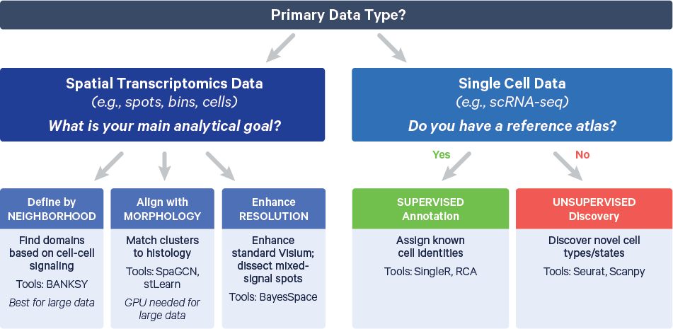
The decision tree below is provided to help you decide the clustering method that best aligns with your data type and research goals:
Obtaining a set of clusters is just the beginning of the interpretation phase. The initial clusters are computational hypotheses that must be rigorously validated and biologically interpreted. This is an iterative process of refinement, where the analyst cycles between clustering, marker identification, and biological annotation to arrive at a meaningful result.
Interactive tools provide a powerful environment for iterative validation, enabling users to visually explore clusters, marker expression, and spatial context in an integrated and intuitive way (see Loupe Browser tutorials for Chromium and Visium data and Xenium Explorer tutorials for Xenium In Situ data).
Step 1: Marker Gene Analysis
The primary method for assigning biological meaning to clusters is to identify marker genes, i.e., genes that are significantly more highly expressed in one cluster compared to all others.
- Finding markers: Standard functions like
FindAllMarkers()in Seurat orsc.tl.rank_genes_groups()in Scanpy perform differential expression tests to identify these genes for each cluster. It is important to view the top markers as the most trustworthy, as p-values can be inflated in single cell data where each cell is treated as a replicate. - Visualizing markers: Data visualization is essential for interpreting marker gene lists:
- Heat maps provide a global view of the top marker genes for every cluster, showing a clear block-diagonal structure if the clustering is robust.
- Violin and dot plots are used to examine the expression of specific, canonical marker genes across all clusters. Violin plots show the full expression distribution, while dot plots concisely convey both the average expression level (color) and the percentage of cells in the cluster expressing the gene (dot size).
- Feature plots overlay the expression of a single gene onto the UMAP or spatial tissue plot. This is arguably the most powerful way to confirm that a marker gene is both specific to and consistently expressed across the cells of a given cluster.
In Loupe Browser, this validation step can be carried out by selecting clusters and overlaying gene expression directly onto UMAP embeddings or spatial tissue images, allowing rapid visual confirmation of cluster specificity and spatial coherence. For more guidance, see the Loupe tutorials on exploring spatial clusters and HD spatial gene expression data. This is often the intuitive way to confirm that a marker gene is both specific to and consistently expressed across the cells of a given cluster.
Step 2: Assigning Cell Identity
With a list of marker genes for each cluster, the next step is annotation. This involves comparing the identified markers to known canonical markers from the literature and public databases (e.g., CellMarker) to assign a biological cell type label to each cluster.
Loupe Browser further supports this process by enabling rapid inspection of canonical marker expression across clusters, which can accelerate biological annotation and validation.
Step 3: The Refinement Loop
The initial annotation often reveals opportunities to refine the clustering.
- Merging clusters: If two or more clusters share a very similar set of marker genes and are adjacent on the UMAP, they likely represent the same cell type that was over-split by the algorithm. The solution is to re-run the clustering at a lower resolution to merge them.
- Splitting and subclustering: Conversely, if a single cluster appears to contain multiple cell types (e.g., it expresses markers for both T cells and B cells) or shows bimodal expression for key genes, it may be under-clustered. The solution is to either increase the resolution or to subset that cluster and re-cluster it on its own—a process known as subclustering—to reveal finer-grained subtypes.
Common Pitfalls and Sanity Checks
A crucial part of validation is using clustering as a tool for anomaly detection. The clusters should not only reflect biology but also reveal potential issues with the data.
- Check for technical confounders: A common pitfall is finding clusters that are defined by technical artifacts rather than biology. A cluster with high expression of only mitochondrial genes likely represents a group of dying cells. A cluster that perfectly separates cells from different experimental batches indicates a strong, uncorrected batch effect. These clusters are not novel cell types and indicate data quality issues that should be addressed.
- Identify the "junk" cluster: It is common to find one or more clusters composed of low-quality cells (low gene counts) or doublets. These should be identified and considered for removal before final interpretation.
- Avoid over-interpretation: Be cautious when interpreting very small clusters. While they could represent a rare cell type, they could also be the result of stochastic noise or a few outlier cells. Their existence should be validated with robust marker expression and, if possible, orthogonal methods.
By treating clusters as hypotheses and using them to probe both the biology and the quality of the data, an analyst can move from a simple computational result to a robust and defensible biological conclusion.