Note: 10x Genomics does not provide support for community-developed tools and makes no guarantees regarding their function or performance. Please contact tool developers with any questions. If you have feedback about Analysis Guides, please email analysis-guides@10xgenomics.com.
We see batch effects between Bright Field (BF) and Immunofluorescence (IF) imaging in Spatial Gene Expression data. Since data are from the same tissues, we would expect gene expression to be similar between sections before staining. Staining should not affect gene expression.
First, we combine Spatial Gene Expression data from two samples from the same tissue, each with a different staining protocol. The data can be combined by running the spaceranger aggr pipeline to combine these data using the following command:
spaceranger aggr --id=staining_IF_BF --csv=IF_BF.csv
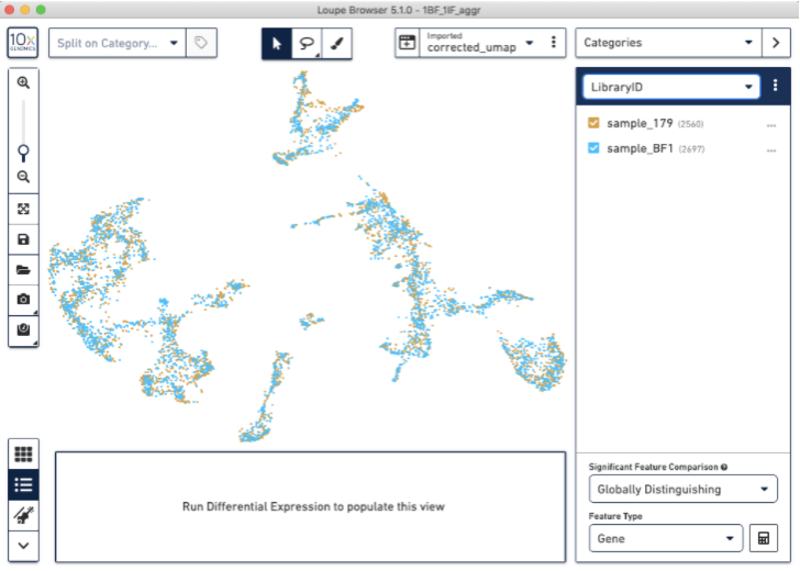
When we load the .cloupe file output from the aggr pipeline into the Loupe Browser, we see this batch effect (see image below) where the two BF (blue) and IF (brown) samples are separated from each other.
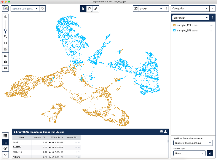
Correcting for this batch effect should bring the cells into alignment.
There are a number of algorithms and tools for correcting batch effects. For more information on batch effects and batch effect correction, see this introduction: Batch Effect Correction.
For this tutorial we are going to use the Harmony batch effect correction algorithm (Korsunsky et al. 2019) implemented in the Seurat R package. The Harmony algorithm is available on GitHub, and the authors of Seurat wrote an integration function in the Seurat package.
If you haven't already installed these libraries, first run these commands to install:
install.packages("dplyr")
install.packages("patchwork")
install.packages("Seurat")
install.packages("cowplot")
install.packages("harmony")
Then load the libraries:
library(dplyr)
library(Seurat)
library(patchwork)
library(cowplot)
library(harmony)
The dataset with the IF filitered matrix can be found here and the dataset with the BF matrix can be found here.
# set working directory to your current location
setwd(".")
# create a local directory called "IF_brain"
dir.create(path = 'IF_brain/')
# set working directory to the newly-created IF_brain directory
setwd("IF_brain")
# download IF filtered matrix:
download.file("https://cf.10xgenomics.com/samples/spatial-exp/1.1.0/V1_Adult_Mouse_Brain_Coronal_Section_1/V1_Adult_Mouse_Brain_Coronal_Section_1_filtered_feature_bc_matrix.tar.gz","V1_Adult_Mouse_Brain_Coronal_Section_1_filtered_feature_bc_matrix.tar.gz")
# decompress the filtered matrix file just downloaded
untar("V1_Adult_Mouse_Brain_Coronal_Section_1_filtered_feature_bc_matrix.tar.gz")
# create a local directory called "BF_brain"
dir.create(path = '../BF_brain/')
setwd("../BF_brain")
download.file("https://cf.10xgenomics.com/samples/spatial-exp/1.1.0/V1_Adult_Mouse_Brain/V1_Adult_Mouse_Brain_filtered_feature_bc_matrix.tar.gz","V1_Adult_Mouse_Brain_filtered_feature_bc_matrix.tar.gz")
untar("V1_Adult_Mouse_Brain_filtered_feature_bc_matrix.tar.gz")
setwd("../")
This section uses commands found in this Seurat vignette. It creates two Seurat objects and merges them together.
Seurat "objects" are a type of data that contain your UMI counts, barcodes, and gene features all in one variable. The Seurat tool has a function called "Read10X()" that will automatically take a directory containing the matrices output from Cell Ranger and input them into the R environment so you don't have to worry about doing this manually. We rely on this function to save us many steps.
We will start by creating two Seurat objects, one for each data set and then take a look at it:
IF_brain.data <- Read10X(data.dir = "IF_brain/filtered_feature_bc_matrix/")
IF_brain<- CreateSeuratObject(counts = IF_brain.data, project = "IF")
IF_brain
BF_brain.data <- Read10X(data.dir = "BF_brain/filtered_feature_bc_matrix/")
BF_brain<- CreateSeuratObject(counts = BF_brain.data, project = "BF")
BF_brain
The output of "BF_brain" and "IF_brain" should be similar:
An object of class Seurat
32285 features across 2702 samples within 1 assay
Active assay: RNA (32285 features, 0 variable features)
Use the merge function to combine the objects. Use the head and the tail functions to check how the data look, to make sure that they are equivalent.
brain.combined <- merge(IF_brain, y = BF_brain, add.cell.ids = c("IF", "BF"), project = "2brains")
head(colnames(brain.combined))
tail(colnames(brain.combined))
The code for creating and merging this object was adapted from the Seurate vignette here.
First, visualize the data before running batch effect correction. Within this command, we will also be normalizing, scaling the data, and calculating gene and feature variance which will be used to run a PCA and UMAP.
brain.combined <- NormalizeData(brain.combined) %>% FindVariableFeatures() %>% ScaleData() %>% RunPCA(verbose = FALSE)
brain.combined <- RunUMAP(brain.combined, dims = 1:30)
DimPlot(brain.combined, group.by = "orig.ident")
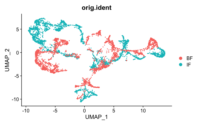
We can see the two samples are not mixed well. But they are better than they were before (see Loupe above). This is probably an effect of normalization, which can help sometimes to correct for small differences.
The next few commands are adapted from the Seurat vignette.
brain.combined <- RunHarmony(brain.combined, group.by.vars = "orig.ident")
brain.combined <- RunUMAP(brain.combined, reduction = "harmony", dims = 1:30)
brain.combined <- FindNeighbors(brain.combined, reduction = "harmony", dims = 1:30) %>% FindClusters()
# "orig.ident" = original identity
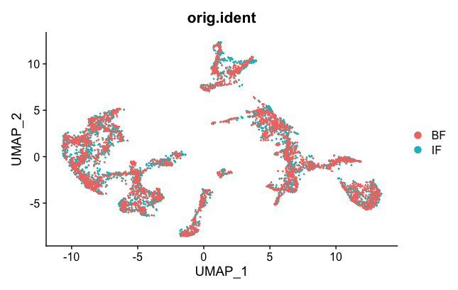
DimPlot(brain.combined, group.by = "orig.ident")
# "ident" = identity, which are clusters
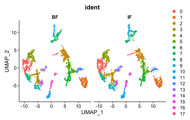
DimPlot(brain.combined, group.by = "ident", split.by = 'orig.ident')
Now the two samples, BF and IF are mixed nicely together. The colors represented in the figure legend are the different clusters. As you can see, they are uniformly spread across the two BF and IF samples now.
Next, we want to export the corrected UMAP projections to a CSV file that can then be loaded into the Loupe Browser. Some of the code was adapted from here.
# split the object
corrected.data <- SplitObject(brain.combined, split.by = "orig.ident")
# edit the barcodes into a format that is compatible with the Loupe Browser
IF.barcode <- rownames(Embeddings(object = corrected.data$IF, reduction = "umap"))
IF.barcode <- gsub("IF_","",IF.barcode)
IF.barcode <- gsub('.{2}$','',IF.barcode)
IF.barcode <- paste(IF.barcode,"-1", sep="")
IF.proj <- Embeddings(object = corrected.data$IF, reduction = "umap")
UMAP.IF <- cbind("Barcode" = IF.barcode, IF.proj)
BF.barcode <- rownames(Embeddings(object = corrected.data$BF, reduction = "umap"))
BF.barcode <- gsub("BF_","",BF.barcode)
BF.barcode <- gsub('.{2}$','',BF.barcode)
BF.barcode <- paste(BF.barcode,"-2", sep="")
BF.proj<- Embeddings(object = corrected.data$BF, reduction = "umap")
UMAP.BF <- cbind("Barcode" = BF.barcode, BF.proj)
# merge the two samples back into the same object, and export into a CSV
corrected.umap <- rbind(UMAP.IF,UMAP.BF)
write.table(corrected.umap, file="corrected_umap.csv", sep = ",", quote = F, row.names = F, col.names = T)
These commands will export the clusters to CSV files that can be loaded into the Loupe Browser.
clusters.IF = Idents(corrected.data$IF)
clusters.IF.data <- cbind("Barcode" = IF.barcode, data.frame("clusters" = clusters.IF))
clusters.BF = Idents(corrected.data$BF)
clusters.BF.data <- cbind("Barcode" = BF.barcode, data.frame("clusters" = clusters.BF))
corrected.cluster <- rbind(clusters.IF.data, clusters.BF.data)
write.table(corrected.cluster, file="corrected_clusters.csv", sep = ",", quote = F, row.names = F, col.names = T)
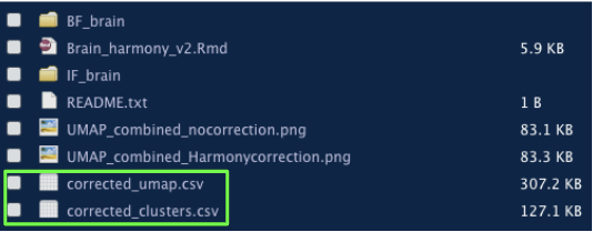
Below we see the two CSV files that were just created.
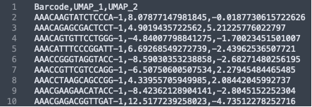
The formatting of the corrected_umap.csv file looks like this:
The formatting of the corrected_clusters.csv looks like this:
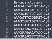
These CSV files have the barcode information of each sample, followed by the new UMAP coordinates and the newly corrected clusters that the barcodes now belong to. The barcodes with a "-1" suffix came from the IF image and the barcodes with the "-2" suffix came from the BF image. When the data from the two images were combined, these suffices were added by the spaceranger aggr pipeline to distinguish which sample the barcodes belong to.
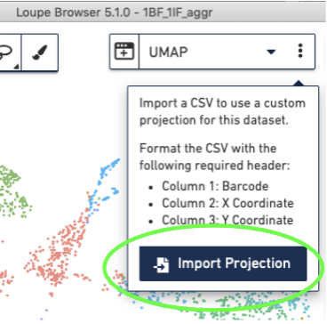
Import the corrected UMAP projections into the Loupe Browser, by selecting the three dots to the right of the UMAP pull-down menu and selecting the "Import Projections" button, and selecting your CSV file:
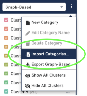
Then import the barcodes associated with the new clusters, by selecting the three dots to the right of the Graph-based cluster Categories and selecting the "Import Categories" button, then selecting your CSV file:
This will give you a new, updated UMAP visualization (new clustering is also available, but not shown):
Now, we have used the Harmony batch effect correction algorithm to better align and re-cluster the barcodes from BF and IF images (note: this tutorial does not modify the count matrix). This batch effect correction removed some of the bias due to technical variation seen between the two staining protocols.