Note: 10x Genomics does not provide support for community-developed tools and makes no guarantees regarding their function or performance. Please contact tool developers with any questions. If you have feedback about Analysis Guides, please email analysis-guides@10xgenomics.com.
Problem: 10x single cell assays typically capture some freely floating transcripts during the droplet-based capture process, resulting in a low level of background RNA counts referred to as ambient RNA. If present in moderate to high levels, ambient RNA can be problematic for downstream analyses for two major reasons: (1) ambient RNA can contaminate the endogenous gene expression profile, confounding cell type annotation results, and (2) differences between conditions may be driven by differences in ambient profiles rather than true biological differences.
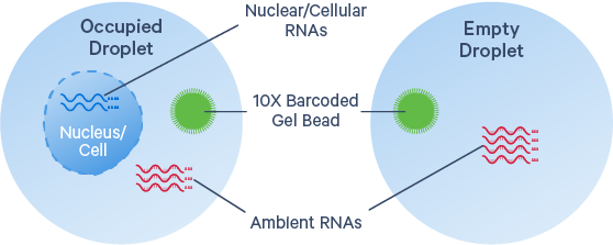
Cause: Background mRNA could derive from cell-free RNA molecules in the cell suspension, ruptured, dead or dying cells, or from other exogenous sources of contamination. High background counts tend to occur more frequently in certain tissue types (Madisson et al., 2019), particularly when working with single cell nuclei samples. The nuclei preparation protocols typically release cytoplasmic RNA into solution (please see our new Chromium Nuclei Isolation product). High debris in such samples will lead to more ambient RNA in the data, but it is still possible to get distinct cell clustering and workable results even without background subtraction.
Solution: While minimizing debris in research samples is important, it must be balanced with the goal of ensuring high-quality samples and avoiding stress or loss of cells and nuclei, which creates a trade-off when attempting to remove ambient RNA. The Cell Ranger cell calling algorithm is effective at distinguishing intact cells from background and filters out non-cell associated reads (see our Algorithms page for more detail). However, in cases where there are high levels of ambient RNA contamination and researchers wish to prioritize higher cell recovery, additional computational approaches may be employed. To computationally identify and remove ambient RNA, one can make use of community-developed tools, which we will highlight in this article below.
One of the first signs that you may need to consider correcting for background RNA is if you get the “Low Fraction Reads in Cells” alert at the top of your Web Summary*:

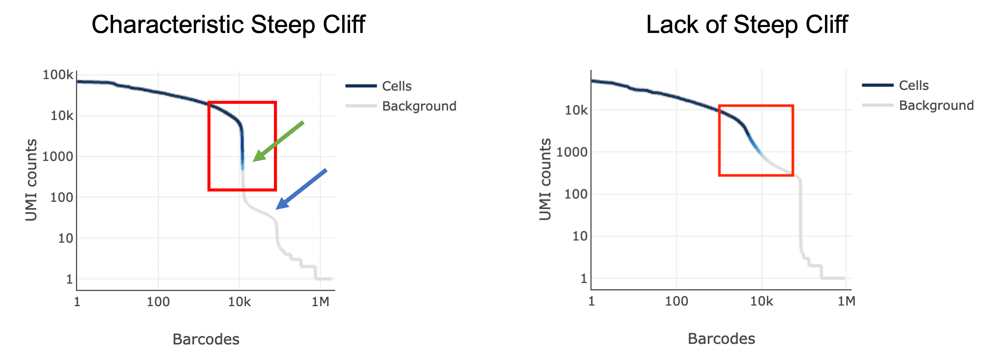
The next thing you might notice in your sample is a barcode rank plot lacking a characteristic “steep cliff” indicating that the algorithm had difficulty in distinguishing cell-containing barcodes from background:
Another potential sign of moderate to high levels of background RNA is enrichment for mitochondrial genes across cluster marker genes, which can be identified in the Web Summary under the “Gene Expression” tab:
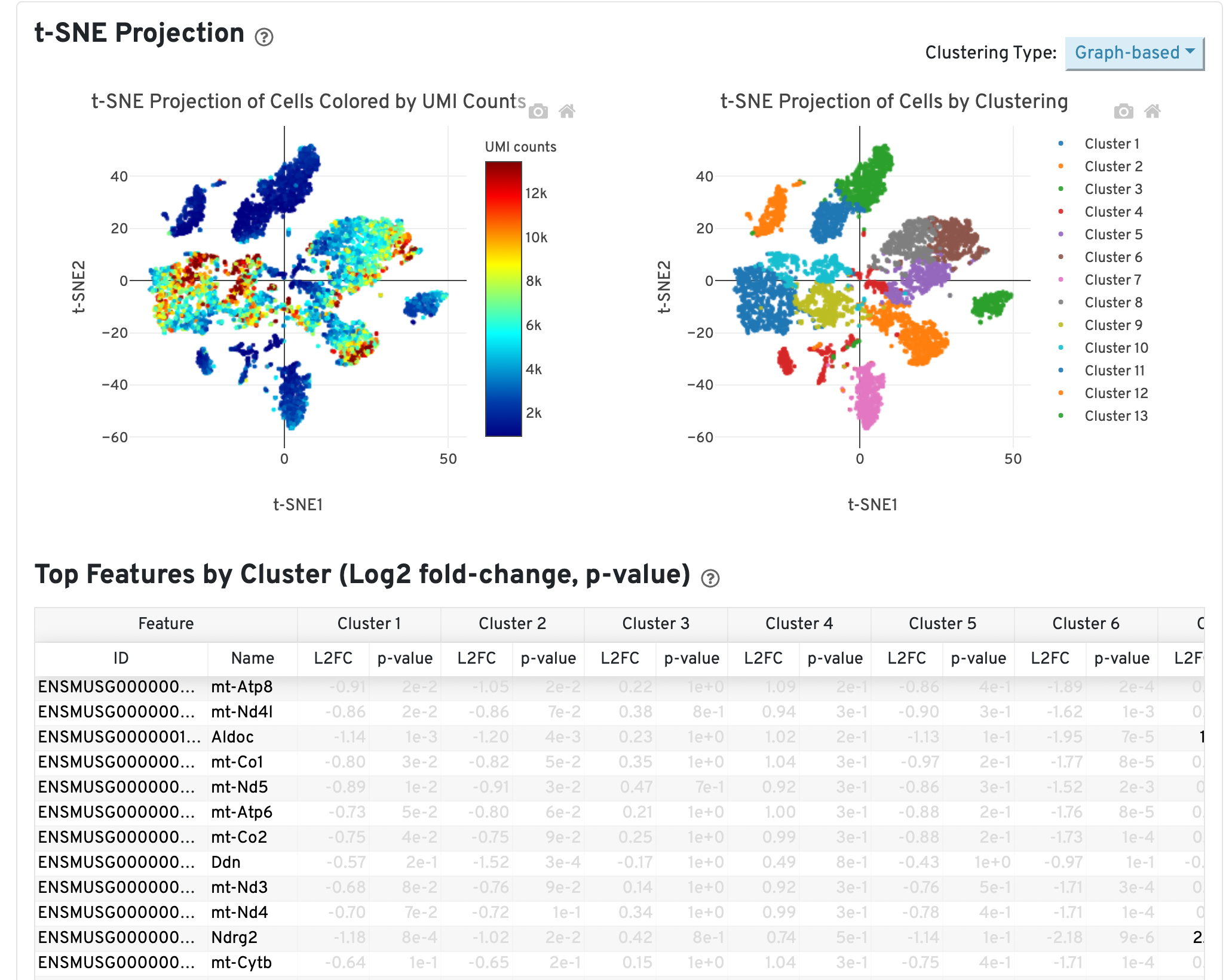
In the example above, genes are sorted by smallest p-value for Cluster 13. This cluster may consist of dead or dying cells or high levels of background RNA originating from cell-free RNAs because mitochondrial genes (genes beginning with “mt-”) are significantly upregulated in this cluster relative to all others.
Ambient RNAs can also originate from more abundant cell types, which can lead to biological misinterpretation when these RNAs contaminate less abundant cell types (Caglayan et al., 2022). This phenomenon can be observed, for example, in mouse brain nuclei, where neuronal markers are observed in glial cell populations and vice versa. Thus, accounting for background RNA profiles often requires a priori knowledge of the sample biology.
As mentioned previously, such data may still be usable even without background subtraction. Whether or not to perform background correction will depend on the extent of contamination and the overall goals of the experiment. For example, one may want to more carefully profile and correct for background contamination using community-developed computational tools if the goal of the experiment is to profile rare cell subtypes. If the overall goals of the experiment involve well-known major cell types, the Cell Ranger cell calling algorithm may perform well enough with its cell calling and filtering steps. Researchers should carefully consider their sample biology, expected cell types, and any unexpected results, such as cell type markers that normally do not overlap co-expressing in one cluster (this may be a sign of ambient RNAs from one cell type partitioning into GEMs as in the neuronal and glial cell type marker example above).
For more information on web summary metrics and recommendations, see our support page and technical note on interpreting web summaries.
* Examples here sourced from Web Summary for 5k Adult Mouse Brain Nuclei isolated with Chromium Nuclei Isolation Kit.
In short, ambient RNA correction can not rescue a failed experiment, for example, in the case of a wetting failure. Wetting failures lead to improper emulsion formation and loss of single cell partitioning, meaning varying numbers of barcoded cells are contained within each GEM, rather than a single barcoded cell per GEM. This can lead to a barcode rank plot that appears suboptimal with a lack of steep cliff similar to what was described above (with some important differences). Researchers may be tempted to try to improve the signal-to-noise ratio of their data by performing ambient RNA correction, however in this case, ambient RNA is not the cause of the poor quality data. Feel free to reach out to 10X Support if you are uncertain about the cause of your suboptimal results and potential solutions.
We do not recommend using ambient RNA correction tools before carefully inspecting your data as suggested above. Not every dataset will require ambient RNA correction; ultimately, this will depend on the experimenters’ goals and knowledge of their sample biology. QC tools, such as ambient RNA correction, often require several iterations of application, modifying parameters, and evaluating the results to see how they impact the data.
Here, we highlight some tools that can computationally identify and remove ambient RNA. We compiled this list based on a combination of factors including citations, quality of documentation, functionality/ease of use, and active support. The list below is not comprehensive. New and exciting tools, algorithms, and other resources continue to be released.
Community-developed tools for background RNA correction generally approach the correction via two mechanisms: removal of empty droplets based on expression profile and removal of ambient RNAs associated with barcodes.
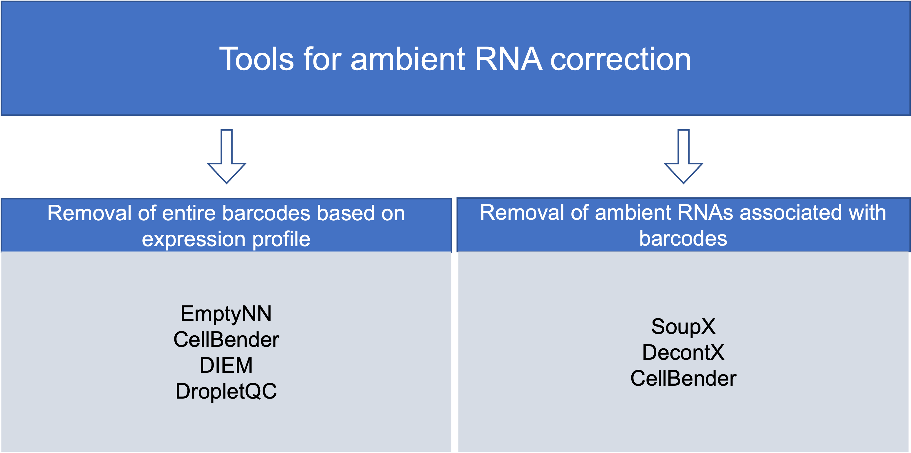
Removing droplets based on expression profile:
EmptyNN (2021): a cell-calling algorithm to identify and remove empty droplets.
- How it works: A neural network is trained to classify cell-free from cell-containing droplets. Barcodes are sorted by UMI count. Low barcodes are defined as the positive set and the rest are the unlabeled set. A subset of the unlabeled set (the higher end of the UMI count) are labeled as cell-containing droplets. The classifier is trained on the positive set and the unlabeled droplets are predicted to either be cell-containing or cell-free over several iterations. Droplets are determined to either be cell-containing or cell-free based on the average prediction over the iterations.
- Programming language: R
- Limitations/considerations: In an analysis of different tools, it failed to call any cells from two datasets (Hodgkin’s lymphoma and glioblastoma), so may not be compatible with all tissue types (Muskovic and Powell, 2021).
- GitHub, Tutorial
CellBender (2019, 2022): a deep generative model that distinguishes cell-containing from cell-free droplets without supervision, learns the profile of background noise, and retrieves a noise-free quantification.
- How it works: A neural network learns the distribution of expression across all droplets in an experiment and estimates the background noise profile of ambient RNAs across all droplets. This tool performs both cell-calling and ambient RNA removal (and so is listed in both categories above). Details and parameters are covered in our CellBender tutorial here.
- Programming language: python
- Limitations/considerations: Relatively heavy computational cost compared to other tools, however use of gpu cuts down on run times significantly.
- GitHub, Tutorial
DIEM (2020): A semi-supervised machine learning classifier that identifies debris on a cell-by-cell basis
- How it works: The software takes as input the raw counts from a single-cell matrix, and the user specifies a subset of barcodes as “fixed debris” based on (1) barcode-rank plot, (2) UMI counts, and (3) % mitochondrial gene expression. After defining the fixed debris droplets and the droplets to be classified, the user then runs differential expression to define the expression profile of debris droplets. The user then initializes the mean parameters with clustering and then runs expectation maximization (EM) to estimate the parameters and classify the droplets. Each droplet is assigned a debris probability and the user can set thresholds to define each droplet as “debris” based on the probability and define whole clusters as “debris clusters” based on the proportion of droplets in each cluster that are defined as debris droplets.
- Programming language: R
- Limitations/considerations: The choice of the cutoff to fix debris and classify droplets is somewhat arbitrary and depends on subjective interpretation of what will likely be included in the debris; the thresholds for determining whether a droplet is debris based on the calculated probability is also arbitrary so there may be a lot of variability in results based on user-defined limits/thresholds.
- GitHub
DropletQC (2021): a method that is able to detect empty droplets, damaged, and intact cells, and accurately distinguish them from one another using a nuclear fraction score.
- How it works: First, the software quantifies, for each droplet, the fraction of RNA originating from unspliced, nuclear pre-mRNA (intronic regions), and uses this to predict whether a droplet is empty, contains a cell, or contains a damaged cell.
- Programming language: R
- Limitations/considerations: Does not remove ambient RNA from barcodes that contain a true cell, and relies on the assumption that ambient RNA consists predominantly of mature cytoplasmic mRNA. However, recent work suggests ambient RNA can come from nuclei and the cytoplasm. The identification of damaged cells is unique to this tool and may be useful for poorer quality datasets.
- GitHub, Tutorial
Removing ambient RNAs associated with barcodes:
SoupX (2020): a method for quantifying the extent of ambient mRNA contamination whilst purifying the true, cell-specific signal from the observed mixture of cellular and exogenous mRNAs.
- How it works: First, the user uploads the unfiltered and filtered barcode-feature matrices so that soupX can define empty droplets. The next step is to estimate the ambient mRNA expression profile from empty droplets. The user can then estimate or manually set the contamination fraction (the fraction of UMIs originating from the background) in each cell. SoupX then corrects the expression of each cell using the ambient mRNA expression profile and estimated contamination.
- Programming language: R
- Limitations/considerations: There are two approaches that customers can use when applying this tool to their data: auto-estimation of the contamination fraction, or manual estimation using a set of known contamination-related genes. This could be a benefit because customers can make use of their knowledge about the biology of their dataset, however, this could add a layer of complexity and the auto estimation may not perform as well as manual.
- GitHub, Tutorial
DecontX (2020): a Bayesian method to estimate and remove contamination in individual cells
- How it works: Assumes the observed expression of a cell is a mixture of counts from two multinomial distributions: (1) a distribution of native transcript counts from the cell’s actual population and (2) a distribution of contaminating transcript counts from all other cell populations captured in the assay. Each cell is treated as a mixture of multinomial distributions over genes, one from its native cell population and another from contamination, and defines the contamination distribution to be a weighted combination of all other cell population distributions. Ultimately, the software deconvolutes a gene-by-cell count matrix and a vector of cell population labels into a matrix of contamination counts and a matrix of native counts, which can then be used in downstream analyses.
- Programming language: R
- Limitations/considerations: Heavily dependent on the accuracy of the clustering provided.
- GitHub, Tutorial
Required skills and resources:
- Ability to program in a scripting language (most commonly R or Python)
- Comfortable in the Linux environment
- Comfortable running command line bioinformatic tools
- Understanding of the tool mechanisms and how it influences analysis
Things to watch out for:
- Applying QC filters and corrections without careful consideration of the data
- Trying to rescue a failed experiment
- Different tools may perform better on different data sets so try a variety of methods