Note: 10x Genomics does not provide support for community-developed tools and makes no guarantees regarding their function or performance. Please contact tool developers with any questions. If you have feedback about Analysis Guides, please email analysis-guides@10xgenomics.com.
Xenium is a new in situ platform from 10x Genomics that quantifies spatial gene expression at subcellular resolution. In addition to automated biochemistry and image acquisition, the platform also performs onboard data analysis so raw images are distilled into data points for cells and transcripts.
As part of the onboard data analysis, Xenium automatically performs nucleus segmentation using a custom neural network. The analysis pipeline takes DAPI signals from the 3D image stack into account but ultimately produces a flattened 2D nucleus segmentation mask. It then expands the nuclear boundary by 5 microns in all directions to approximate the cell boundary, and assigns transcripts to a cell if it falls within the cell boundary.
Because the Xenium cell segmentation mask is 2D, transcripts are assigned to extruded 2D shapes, based solely on their x and y coordinates. The net result is akin to using cookie cutters on a thin layer of cookie dough.

Customers may wish to perform their own cell segmentation using a third-party tool if they are not satisfied with Xenium's default cell segmentation and transcript mapping. Xenium Ranger allows importing of 2D third-party segmentation results to create a Xenium bundle that can be explored in Xenium Explorer and read by most spatial and single-cell analysis packages. For true 3D segmentation this analysis guide uses Cellpose 2.1 and provides a path to create a feature-cell matrix that can be used for downstream data analysis.
This analysis guide requires the following 2 files from the Xenium output folder:
- morphology.ome.tif
- transcripts.parquet
Once the requisite libraries are installed, the first section will show how to perform nucleus segmentation with Cellpose 2.1 using Xenium's DAPI TIFF image. The result will be a numpy data dictionary (*.ome_seg.npy) and a nuclei masked image (*.ome_cp_masks.tif).
The second section will show how to combine transcripts' 3D locations (from transcripts.parquet) with Cellpose nucleus segmentation results to assign transcripts to cells using custom code. The final result is a feature-cell matrix in MTX format that is compatible with popular third-party tools such as Seurat and Scanpy.
Miniconda
This article will use a wide variety of third-party Python libraries. We recommend using Miniconda to install them, in addition to creating two conda environments that will be used throughout this guide. Miniconda can be installed by following the directions at: https://docs.conda.io/projects/conda/en/latest/user-guide/install/index.html
Python Libraries
tifffilelibrary is popular for reading and writing TIFF image files. In particular, it supports the OME-TIFF multi-page format that is produced by Xenium.pyarrowlibrary will be used to read files in Apache Parquet format.pandaslibrary has data structures that make it easy to work with mixed type tabular data.scipylibrary has support for sparse matrices and it will be used to produce a feature-cell matrix in MTX format.
These libraries can be installed by running the following shell commands
# Update conda
conda update conda
# Create the xenium conda environment
conda create --name xenium python=3.9.12
# Activate the xenium conda environment
conda activate xenium
# Install libraries
conda install tifffile
conda install -c conda-forge pyarrow
conda install pandas
conda install scipy
# Go back to base environment
conda deactivate
After running the commands above, you should now have a xenium conda environment with the following installed:
python3.9.12tifffile2021.7.2pyarrow4.0.0pandas1.4.3scipy1.7.3
Cellpose 2.1
Cellpose is a generalist algorithm for segmentation. The website at https://www.cellpose.org/ has a drag and drop UI, but it is limited for several reasons:
- Only runs the older Cellpose 1.0
- Input image is limited to <10MB, and up to 512x512 pixels.
Due to the aforementioned limitations, we will install the Python library and create a script to perform nucleus segmentation. Cellpose 2.1 installation steps are documented here, and summarized by the following shell commands:
conda create --name cellpose python=3.8
# Activate the cellpose environment
conda activate cellpose
# Install Cellpose
python -m pip install cellpose
# Go back to base environment
conda deactivate
You should now have a cellpose conda environment with the following installed:
python3.8.13cellpose2.1.0
File Format Overview – morphology.ome.tif
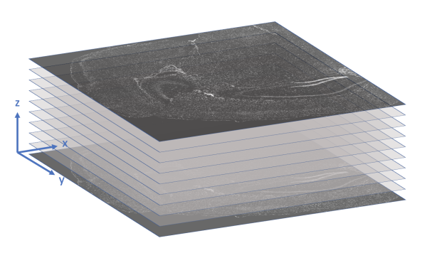
The morphology.ome.tif image produced by Xenium is an image pyramid that contains 7 copies of the image stack at varying resolutions. Each level contains a 3D image stack with approximately 10 z-slices This concept is illustrated in the following figure.
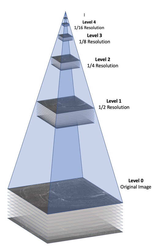
Here's a video game analogy to explain the rationale behind the image pyramid. In games, 3D models often have variable levels of detail (LOD). Up close, a character model may consist of thousands of polygons. However, when that same character is 1/4 mile away in the game world, it can probably be represented by <100 polygons, and players won’t notice the reduction in detail. This makes it more efficient to render the whole scene.
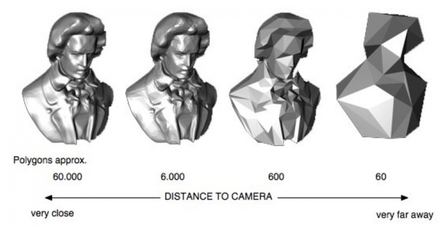
Image generated using OpenSG 2 Vision.
With Xenium Explorer, the browser pulls from different levels of morphology.ome.tif depending on the level of zoom, and displays only what you need to see to remain quick and responsive despite the torrent of data. If you are looking at the whole tissue, you can probably get by with one of the lower resolution images.
Extract a Single Level from morphology.ome.tif
Cellpose can handle a 3D image stack with (x, y, z) info, but it is not compatible with an image pyramid. As such, it is necessary to extract a single level from morphology.ome.tif before proceeding further.
The choice of level will affect the segmentation result. A higher resolution input will result in more detailed segmentation at the cost of longer runtime.
| Input Resolution | 10 x 1424 x 1550 | 10 x 5696 x 6200 |
|---|---|---|
| Segmentation Result | 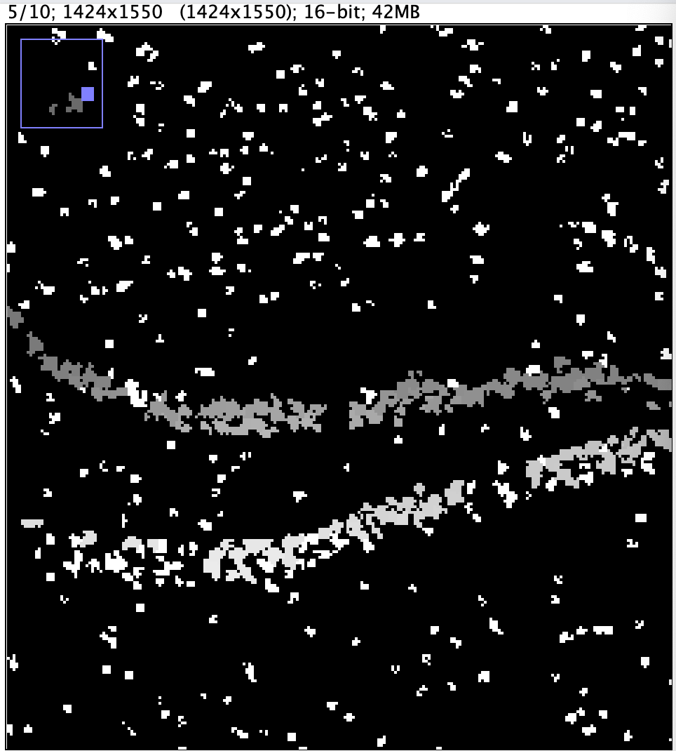 | 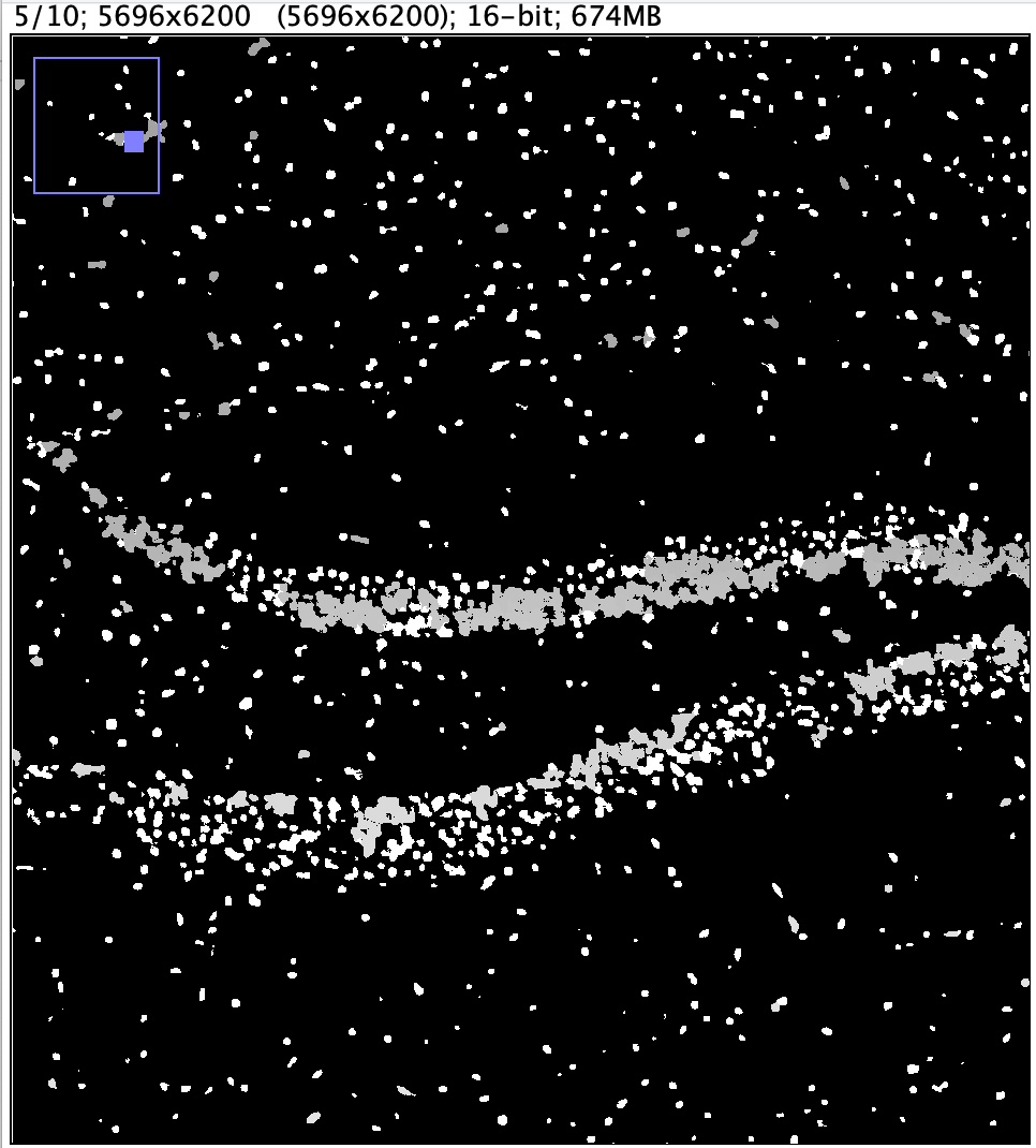 |
| Segmentation Runtime | 162 min. 55 sec. | 300 min. 34 sec. |
Once you decide which level to extract, the following Python script can be used to pull out a specific level, and save it as a separate image. To run the script, please do the following:
- Copy and paste the code to a new text file.
#!/usr/bin/env python
import tifffile
# Variable 'LEVEL' determines the level to extract. It ranges from 0 (highest
# resolution) to 6 (lowest resolution) for morphology.ome.tif
LEVEL = 2
with tifffile.TiffFile('morphology.ome.tif') as tif:
image = tif.series[0].levels[LEVEL].asarray()
tifffile.imwrite(
'level_'+str(LEVEL)+'_morphology.ome.tif',
image,
photometric='minisblack',
dtype='uint16',
tile=(1024, 1024),
compression='JPEG_2000_LOSSY',
metadata={'axes': 'ZYX'},
)
- Modify the LEVEL variable (line 7) to the desired value.
- Save the file with a *.py extension (e.g. extract_tiff.py).
- Give the script execute permission.
# Give files with .py extension execute permission
chmod 755 *.py
- Activate the xenium conda environment before running the script.
# Activate the xenium conda environment
conda activate xenium
# Run Python script
./extract_tiff.py
Running Cellpose 2.1
Command-line options for Cellpose are documented at https://cellpose.readthedocs.io/en/latest/command.html#command-line-examples. In particular, we want to highlight these parameters:
--use_gpu: If you have access to a machine with GPU, there is potential for performance improvement. We did not test this option, and all runtimes provided in this analysis guide come from running Cellpose on a standard server.--pretrained_model nuclei: During testing, we did not try training our own model; we used the pre-trained nuclei model. Cellpose will automatically download the model the first time you use it.--do_3D: Cellpose is able to perform 3D segmentation. Xenium outputs an image stack with approximately 10 z-slices that are spaced 3 microns apart, so we enable this option.--diameter: This parameter specifies target diameter in pixels, and can greatly affect segmentation results. Unfortunately, Cellpose is not able to automatically estimate a value when it is run in 3D mode, so some experimentation is needed to determine the optimal setting. In the table below, you can see how much segmentation results and runtimes can vary, given an identical Level 2 input image.
--diameter setting | 8 | 16 | 24 |
|---|---|---|---|
| Segmentation Result | 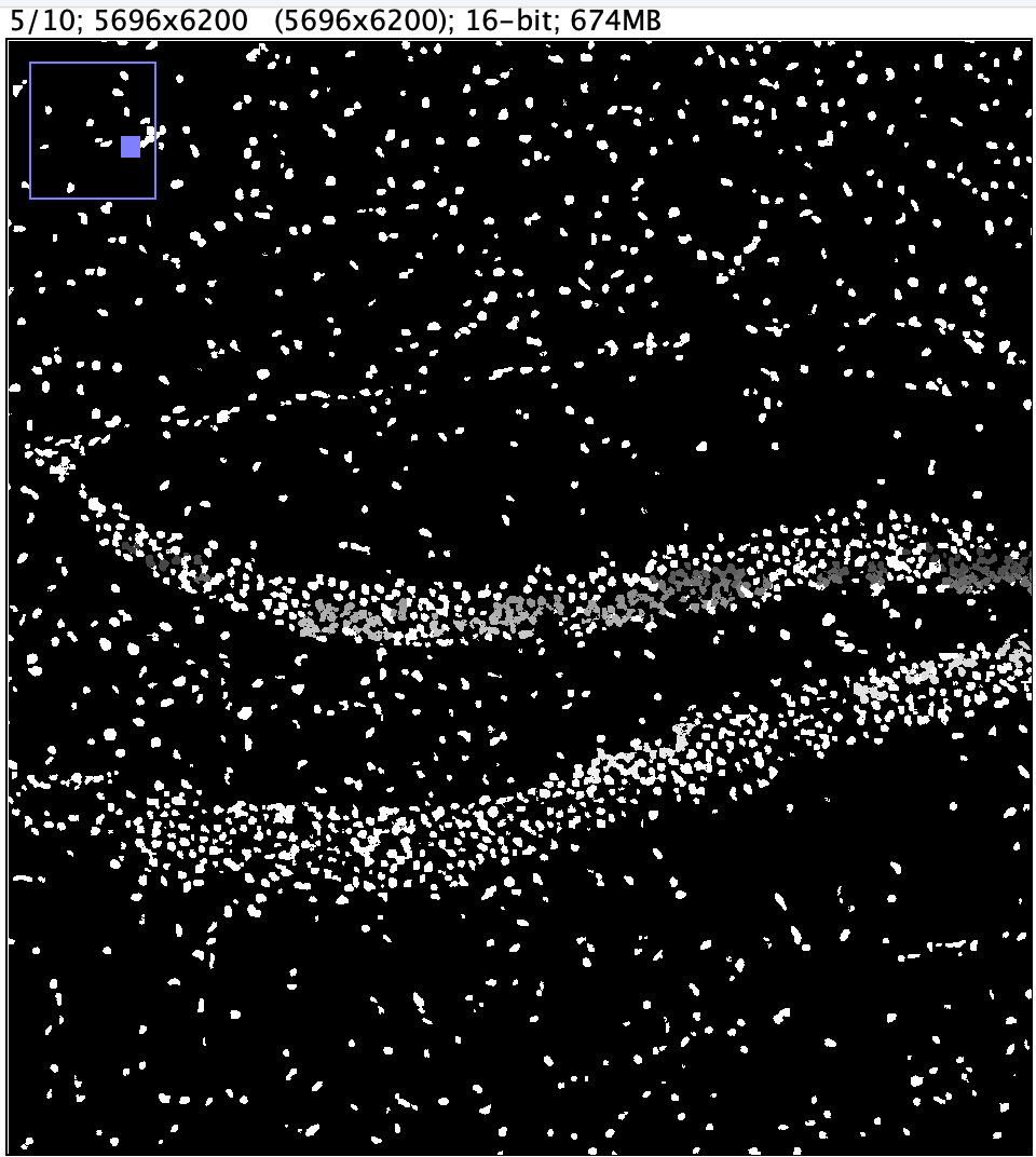 |  | 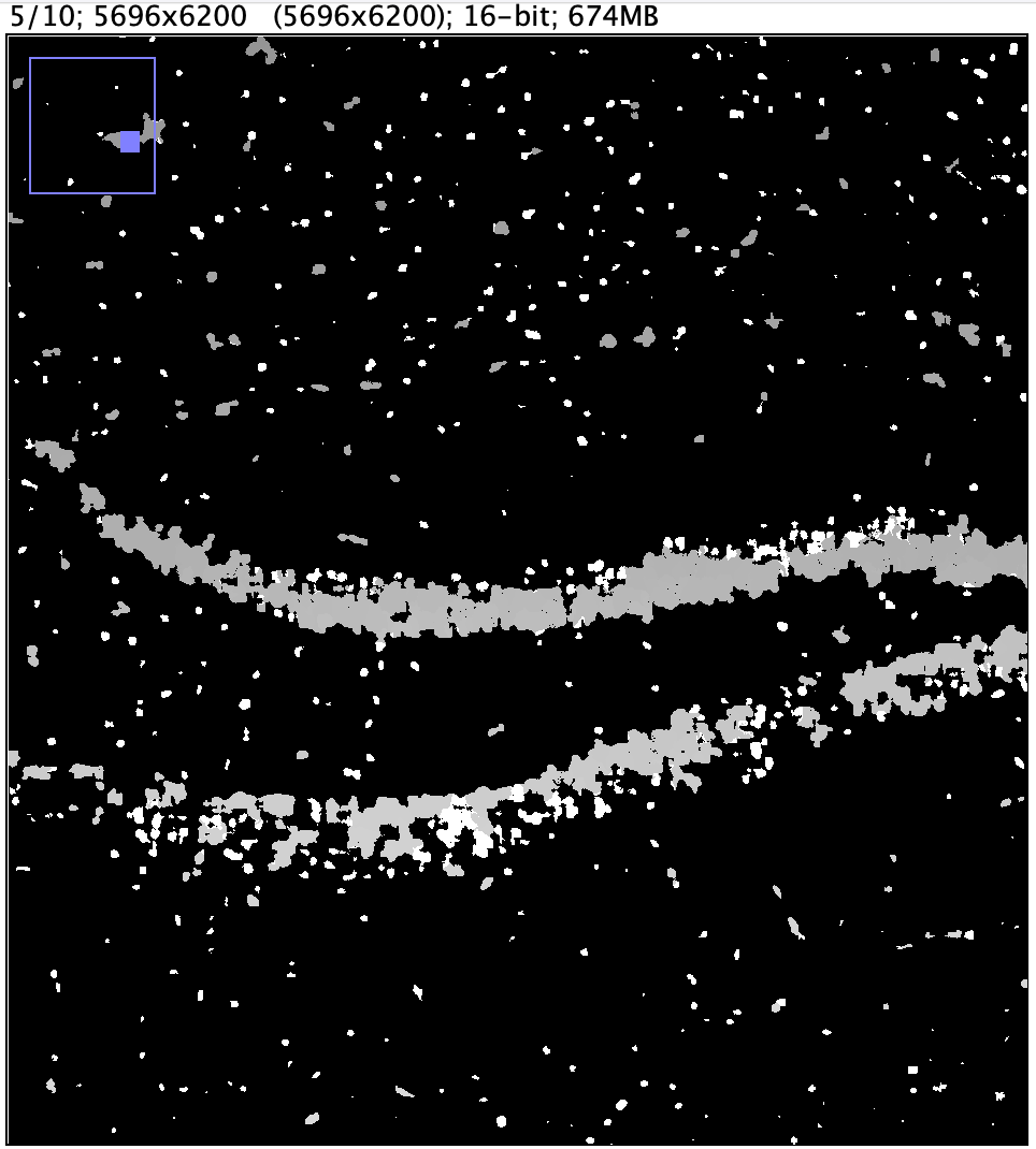 |
| Segmentation Runtime | 788 min. 50 sec. | 300 min. 34 sec. | 300 min. 35 sec. |
For mouse brain data, setting the --diameter parameter to 7-10 microns seems to yield good results. The optimal setting will obviously vary with other types of tissue, and it's important to convert the target diameter from microns to pixels, depending on which level was extracted from the image pyramid.
The following python script will print out the image description of morphology.ome.tif. This script should be run using the xenium conda environment.
#!/usr/bin/env python
import tifffile
with tifffile.TiffFile('morphology.ome.tif') as tif:
for tag in tif.pages[0].tags.values():
if tag.name == "ImageDescription":
print(tag.name+":", tag.value)
In particular, the description includes the following line showing that at level 0, each pixel is 0.2125 micron x 0.2125 micron in (x, y).
<Pixels DimensionOrder="XYZCT" ID="Pixels:0" SizeC="1" SizeT="1" SizeX="22784" SizeY="24800" SizeZ="10" Type="uint16" PhysicalSizeX="0.2125" PhysicalSizeY="0.2125" PhysicalSizeZ="3.0">
With that information, here is a table that lists pixel size at various levels of the image pyramid:
| Level | Pixel size (micron) |
|---|---|
| 0 | 0.2125 |
| 1 | 0.425 |
| 2 | 0.85 |
| 3 | 1.7 |
| 4 | 3.4 |
| 5 | 6.8 |
| 6 | 13.6 |
Putting everything together, the following is a sample Cellpose command that can be run from the shell:
# Activate the cellpose environment
conda activate cellpose
# Cellpose 2.1 command
python -m cellpose --dir <ABS_PATH_OF_IMG> --pretrained_model nuclei --chan 0 --chan2 0 --img_filter _morphology.ome --diameter <DIAMETER_PIXEL> --do_3D --save_tif --verbose
# Deactivate cellpose environment
conda deactivate
OverflowError: serializing a bytes object larger than 4 GiB requires pickle protocol 4 or higherUltimately, this error is caused by a known issue in numpy (https://github.com/numpy/numpy/issues/18784) which hard-codes the use of pickle protocol 3. The newer protocol 4 has been available since Python 3.4, and because we specified Python 3.8 in the cellpose conda environment, it should be possible to use protocol 4 and circumvent the 4GB file size limitation. Let's go ahead and make a minor source code modification to numpy.
First, find where your numpy library is installed by running the following shell command. It will display directories where Python libraries are found:
conda activate cellpose
python -c "import sys; print(sys.path)"
If you use Miniconda to install Python libraries, and set up a cellpose conda environment as suggested above, the file that needs to be edited should be located at <SOME_PATH_PREFIX>/miniconda3/envs/cellpose/lib/python3.8/site-packages/numpy/lib/format.py
Use your favorite text editor, and change line 679 of format.py, located in the write_array() function,
FROM
pickle.dump(array, fp, protocol=3, **pickle_kwargs)
TO
pickle.dump(array, fp, protocol=pickle.HIGHEST_PROTOCOL, **pickle_kwargs)
File Format Overview – transcripts.parquet
Xenium outputs transcript data in 3 different formats:
- transcripts.csv.gz
- transcripts.parquet
- transcripts.zarr.zip
Depending on the choice of downstream analysis tools, one format may be easier or faster to process than another.
This article will focus on the Apache Parquet file format. Unlike the row-based CSV format where data is stored line by line (row by row), Parquet is column-based. Because data in each column usually share the same data type, Parquet files can be compressed and decompressed very efficiently. In general, this modern file format is much smaller and faster relative to CSV. For a more in-depth comparison between Parquet and CSV, please take a look at this article.
Use the following python script to quickly determine the column names and their associated data types in transcripts.parquet. The script will also print out the first 10 records. Please run this script using the xenium conda environment.
#!/usr/bin/env python3
import pandas as pd
data_frame = pd.read_parquet('transcripts.parquet')
print(data_frame.dtypes)
print(data_frame[:10])
Running the python script returns the following, showing that transcripts.parquet contains 8 columns.
transcript_id uint64
cell_id int32
overlaps_nucleus uint8
feature_name object
x_location float32
y_location float32
z_location float32
qv float32
dtype: object
transcript_id cell_id overlaps_nucleus feature_name x_location y_location z_location qv
0 281474976710656 153 1 b'Chst9' 467.284912 723.035156 10.867549 13.371499
1 281474976710657 85 1 b'Bhlhe40' 618.211121 717.488708 14.101116 12.122915
2 281474976710658 191 0 b'Wfs1' 598.623840 782.937134 13.952497 40.000000
3 281474976710659 203 0 b'Wfs1' 610.280945 798.482544 13.899248 40.000000
4 281474976710660 199 0 b'Dkk3' 532.640747 800.270020 14.038778 40.000000
5 281474976710661 205 0 b'Gjb2' 412.885162 813.587158 13.887715 40.000000
6 281474976710662 -1 0 b'Dkk3' 535.707947 861.141846 14.190361 12.725308
7 281474976710663 -1 0 b'Lyz2' 340.266418 865.291199 13.883341 40.000000
8 281474976710664 -1 0 b'Car4' 211.336823 879.179504 13.700431 40.000000
9 281474976710665 1342 0 b'Lyz2' 367.774048 890.858215 13.799179 40.000000
Here are a few quick notes about some of these columns:
- cell_id: If a transcript is not associated with a cell, it will get -1. Cell assignment is based on Xenium's default 2D segmentation mask, and is likely irrelevant if we want to use the 3D segmentation result from Cellpose.
- x_location, y_location, z_location: These 3 columns store the (x, y, z) coordinates of the transcript in microns. The origin is found in the upper-left corner of the bottom z-slice, as the following image illustrates.
- qv: Phred-scaled quality score of all decoded transcripts. It is up to the customer to determine a suitable Q-Score threshold when analyzing Xenium data. At 10x Genomics, we typically filter out transcripts with Q-Score < 20.
Reading Cellpose Segmentation Mask
Cellpose produces a *.ome_seg.npy output file that contains the nucleus segmentation results. This file is documented on https://cellpose.readthedocs.io/en/latest/outputs.html.
It is also possible to list all the keys, the datatypes, and dimensions using the following python script. Please run this script using the xenium conda environment.
#!/usr/bin/env python3
import numpy as np
from glob import glob
fnames = glob('*morphology.ome_seg.npy')
for f in fnames:
dat = np.load(f, allow_pickle=True).item()
for key in dat.keys():
dtype = type(dat[key])
print("Key:", key)
print("Dtype:", dtype)
if isinstance(dat[key], np.ndarray):
print("Dimension:", dat[key].shape)
elif isinstance(dat[key], list):
print("Length:", len(dat[key]))
# empty line between keys
print()
Running the script above would produce an output such as the following:
Key: outlines
Dtype: <class 'numpy.ndarray'>
Dimension: (12, 3125, 2861)
Key: masks
Dtype: <class 'numpy.ndarray'>
Dimension: (12, 3125, 2861)
Key: chan_choose
Dtype: <class 'list'>
Length: 2
Key: img
Dtype: <class 'numpy.ndarray'>
Dimension: (12, 3125, 2861)
Key: ismanual
Dtype: <class 'numpy.ndarray'>
Dimension: (32845,)
Key: filename
Dtype: <class 'str'>
Key: flows
Dtype: <class 'list'>
Length: 5
Key: est_diam
Dtype: <class 'float'>
Of these, the ndarray stored under the "masks" key will be most relevant to us, since every (z-slice, y-pixel, x-pixel) in the original image that is given to Cellpose will be assigned to a unique cell ID. If 0 is assigned, then that location is dark in the original image and is not associated with a cell based on DAPI nucleus segmentation.
Mapping Transcripts
Putting everything together, the Python script below will perform these tasks:
- Process all transcripts from transcripts.parquet, and assign them to cells based on Cellpose nucleus segmentation results.
- Perform a neighborhood search for unassigned transcripts. Since Cellpose only performs nucleus segmentation from DAPI signals, many transcripts that are located in the cytoplasm will be in unassigned space. The script uses a heuristic that associates those transcripts with the nearest nucleus if the Euclidean distance is within a user-specified limit. The default nuclear expansion distance is 10 microns, and this can be adjusted via the
-nuc_expparameter. - Generate a feature-cell matrix and output that matrix in MTX format that is compatible with Seurat and Scanpy.
Running the script with -h would display the help text that lists the required and optional parameters. This script should be run using the xenium conda environment. It's also important to specify the correct -pix_size argument depending on the level that was extracted from the image pyramid in the nucleus segmentation section.
#!/usr/bin/env python3
import argparse
import csv
import os
import sys
import numpy as np
import pandas as pd
import re
import scipy.sparse as sparse
import scipy.io as sio
import subprocess
# Define constant.
# z-slices are 3 microns apart in morphology.ome.tif
Z_SLICE_MICRON = 3
def main():
# Parse input arguments.
args = parse_args()
# Check for existence of input file.
if (not os.path.exists(args.cellpose)):
print("The specified Cellpose output (%s) does not exist!" % args.cellpose)
sys.exit(0)
if (not os.path.exists(args.transcript)):
print("The specified transcripts.parquet file (%s) does not exist!" % args.transcript)
sys.exit(0)
# Check if output folder already exist.
if (os.path.exists(args.out)):
print("The specified output folder (%s) already exists!" % args.out)
sys.exit(0)
# Define additional constants
NUC_EXP_PIXEL = args.nuc_exp / args.pix_size
NUC_EXP_SLICE = args.nuc_exp / Z_SLICE_MICRON
# Read Cellpose segmentation mask
seg_data = np.load(args.cellpose, allow_pickle=True).item()
mask_array = seg_data['masks']
# Use regular expression to extract dimensions from mask_array.shape
m = re.match("\((?P<z_size>\d+), (?P<y_size>\d+), (?P<x_size>\d+)", str(mask_array.shape))
mask_dims = { key:int(m.groupdict()[key]) for key in m.groupdict() }
# Read 5 columns from transcripts Parquet file
transcripts_df = pd.read_parquet(args.transcript,
columns=["feature_name",
"x_location",
"y_location",
"z_location",
"qv"])
# Find distinct set of features.
features = np.unique(transcripts_df["feature_name"])
# Create lookup dictionary
feature_to_index = dict()
for index, val in enumerate(features):
feature_to_index[str(val, 'utf-8')] = index
# Find distinct set of cells. Discard the first entry which is 0 (non-cell)
cells = np.unique(mask_array)[1:]
# Create a cells x features data frame, initialized with 0
matrix = pd.DataFrame(0, index=range(len(features)), columns=cells, dtype=np.int32)
# Iterate through all transcripts
for index, row in transcripts_df.iterrows():
if index % args.rep_int == 0:
print(index, "transcripts processed.")
feature = str(row['feature_name'], 'utf-8')
x = row['x_location']
y = row['y_location']
z = row['z_location']
qv = row['qv']
# Ignore transcript below user-specified cutoff
if qv < args.qv_cutoff:
continue
# Convert transcript locations from physical space to image space
x_pixel = x / args.pix_size
y_pixel = y / args.pix_size
z_slice = z / Z_SLICE_MICRON
# Add guard rails to make sure lookup falls within image boundaries.
x_pixel = min(max(0, x_pixel), mask_dims["x_size"] - 1)
y_pixel = min(max(0, y_pixel), mask_dims["y_size"] - 1)
z_slice = min(max(0, z_slice), mask_dims["z_size"] - 1)
# Look up cell_id assigned by Cellpose. Array is in ZYX order.
cell_id = mask_array[round(z_slice)] [round(y_pixel)] [round(x_pixel)]
# If cell_id is 0, Cellpose did not assign the pixel to a cell. Need to perform
# neighborhood search. See if nearest nucleus is within user-specified distance.
if cell_id == 0:
# Define neighborhood boundary for 3D ndarray slicing. Take image boundary into
# consideration to avoid negative index.
z_neighborhood_min_slice = max(0, round(z_slice-NUC_EXP_SLICE))
z_neighborhood_max_slice = min(mask_dims["z_size"], round(z_slice+NUC_EXP_SLICE+1))
y_neighborhood_min_pixel = max(0, round(y_pixel-NUC_EXP_PIXEL))
y_neighborhood_max_pixel = min(mask_dims["y_size"], round(y_pixel+NUC_EXP_PIXEL+1))
x_neighborhood_min_pixel = max(0, round(x_pixel-NUC_EXP_PIXEL))
x_neighborhood_max_pixel = min(mask_dims["x_size"], round(x_pixel+NUC_EXP_PIXEL+1))
# Call helper function to see if nearest nucleus is within user-specified distance.
cell_id = nearest_cell(args, x_pixel, y_pixel, z_slice,
x_neighborhood_min_pixel,
y_neighborhood_min_pixel,
z_neighborhood_min_slice,
mask_array[z_neighborhood_min_slice : z_neighborhood_max_slice,
y_neighborhood_min_pixel : y_neighborhood_max_pixel,
x_neighborhood_min_pixel : x_neighborhood_max_pixel])
# If cell_id is not 0 at this point, it means the transcript is associated with a cell
if cell_id != 0:
# Increment count in feature-cell matrix
matrix.at[feature_to_index[feature], cell_id] += 1
# Call a helper function to create Seurat and Scanpy compatible MTX output
write_sparse_mtx(args, matrix, cells, features)
#--------------------------
# Helper functions
def parse_args():
"""Parses command-line options for main()."""
summary = 'Map Xenium transcripts to Cellpose segmentation result. \
Generate Seurat/Scanpy-compatible feature-cell matrix.'
parser = argparse.ArgumentParser(description=summary)
requiredNamed = parser.add_argument_group('required named arguments')
requiredNamed.add_argument('-cellpose',
required = True,
help="The path to the *.ome_seg.npy file produced " +
"by Cellpose.")
requiredNamed.add_argument('-transcript',
required = True,
help="The path to the transcripts.parquet file produced " +
"by Xenium.")
requiredNamed.add_argument('-out',
required = True,
help="The name of output folder in which feature-cell " +
"matrix is written.")
requiredNamed.add_argument('-pix_size',
required = True,
type=float,
help="The size of each pixel, in microns, for the " +
"image that is passed to Cellpose for nucleus " +
"segmentation.")
parser.add_argument('-nuc_exp',
default='10.0',
type=float,
help="The expansion distance from the nuclear boundary, " +
"in microns, for cell boundary. (default: 10.0)")
parser.add_argument('-qv_cutoff',
default='20.0',
type=float,
help="Ignore transcripts with QV score below this " +
"threshold. (default: 20.0)")
parser.add_argument('-rep_int',
default='10000',
type=int,
help="Reporting interval. Will print message to stdout " +
"whenever the specified # of transcripts is processed. " +
"(default: 10000)")
try:
opts = parser.parse_args()
except:
sys.exit(0)
return opts
def nearest_cell(args, x_pixel, y_pixel, z_slice,
x_neighborhood_min_pixel, y_neighborhood_min_pixel,
z_neighborhood_min_slice, mask_array):
"""Check if nearest nucleus is within user-specified distance.
If function returns 0, it means no suitable nucleus was found."""
# Initialize constants
NUC_EXP_PIXEL = args.nuc_exp / args.pix_size
# For Euclidean distance, we need to convert z-slice to z-micron
SLICE_TO_PIXEL = Z_SLICE_MICRON / args.pix_size
# When we take a neighborhood slice of mask_array, all indices start at (0,0,0).
# This INDEX_SHIFT is necessary to reconstruct coordinates from original mask_array.
INDEX_SHIFT = np.array([z_neighborhood_min_slice,
y_neighborhood_min_pixel,
x_neighborhood_min_pixel])
min_dist = NUC_EXP_PIXEL
cell_id = 0
# Enumerate through all points in the neighborhood
for index, cell in np.ndenumerate(mask_array):
# Current point is not assigned to a nucleus.
if cell == 0:
continue
# Current point IS assigned to a nucleus. But is it within NUC_EXP_PIXEL?
else:
img_loc = np.asarray(index, dtype=float) + INDEX_SHIFT
# Convert from z-slice to "z-pixel"
img_loc[0] *= SLICE_TO_PIXEL
transcript_loc = np.array([z_slice * SLICE_TO_PIXEL, y_pixel, x_pixel])
# Calculate Euclidean distance between 2 points
dist = np.linalg.norm(transcript_loc - img_loc)
if dist < min_dist:
min_dist = dist
cell_id = cell
return cell_id
def write_sparse_mtx(args, matrix, cells, features):
"""Write feature-cell matrix in Seurat/Scanpy-compatible MTX format"""
# Create the matrix folder.
os.mkdir(args.out)
# Convert matrix to scipy's COO sparse matrix.
sparse_mat = sparse.coo_matrix(matrix.values)
# Write matrix in MTX format.
sio.mmwrite(args.out + "/matrix.mtx", sparse_mat)
# Write cells as barcodes.tsv. File name is chosen to ensure
# compatibility with Seurat/Scanpy.
with open(args.out + "/barcodes.tsv", 'w', newline='') as tsvfile:
writer = csv.writer(tsvfile, delimiter='\t', lineterminator='\n')
for cell in cells:
writer.writerow(["cell_" + str(cell)])
# Write features as features.tsv. Write 3 columns to ensure
# compatibility with Seurat/Scanpy.
with open(args.out + "/features.tsv", 'w', newline='') as tsvfile:
writer = csv.writer(tsvfile, delimiter='\t', lineterminator='\n')
for f in features:
feature = str(f, 'utf-8')
if feature.startswith("NegControlProbe_") or feature.startswith("antisense_"):
writer.writerow([feature, feature, "Negative Control Probe"])
elif feature.startswith("NegControlCodeword_"):
writer.writerow([feature, feature, "Negative Control Codeword"])
elif feature.startswith("BLANK_"):
writer.writerow([feature, feature, "Blank Codeword"])
else:
writer.writerow([feature, feature, "Gene Expression"])
# Seurat expects all 3 files to be gzipped
subprocess.run("gzip -f " + args.out + "/*", shell=True)
if __name__ == "__main__":
main()
If the script above is saved to a file called map_transcripts.py, then a sample invocation might look like the following:
# Activate the xenium conda environment
conda activate xenium
# Map transcripts to cells
./map_transcripts.py -cellpose level_3_morphology.ome_seg.npy -transcript transcripts.parquet -out feature_cell_matrix -pix_size 1.7
The script spends the majority of time performing neighborhood searches, so the choice of -nuc_exp will greatly impact overall runtime. Larger nuclear expansion distances will allow more transcripts to be associated with a cell, but we expect a roughly cubic growth in runtime since neighborhoods expand in 3 dimensions.
The table below shows the relationship between nuclear expansion distance, cell-associated Q20 transcripts, and script runtime. These results are based on processing the first million transcripts, 806,508 of which have Q-Score >= 20, from a mouse brain dataset. Depending on the nuclear expansion distance, different numbers of transcripts can be associated with a cell (cell-associated Q20 transcript) as shown in the table below. The whole dataset has almost 20 million decoded transcripts, so we can expect a twenty-fold increase in runtime to map all transcripts in this mouse brain sample.
| Nuclear Expansion Distance | Cell-Associated Q20 Transcripts | Script Runtime |
|---|---|---|
| 0 micron | 49,846 | 2 min. 23 sec. |
| 5 microns | 98,031 | 12 min. 24 sec. |
| 10 microns | 125,874 | 60 min. 14 sec. |
| 15 microns | 139,917 | 165 min. 7 sec. |
After running the Python transcript mapping script, the resulting feature-cell matrix can be read by popular third-party tools such as Seurat and Scanpy.
To demonstrate compatibility, we were able to follow this Seurat vignette and use the Read10X() function to load the matrix. We produced the following plots, and it should be straightforward to cluster the cells, generate a UMAP projection, and find differentially expressed features.
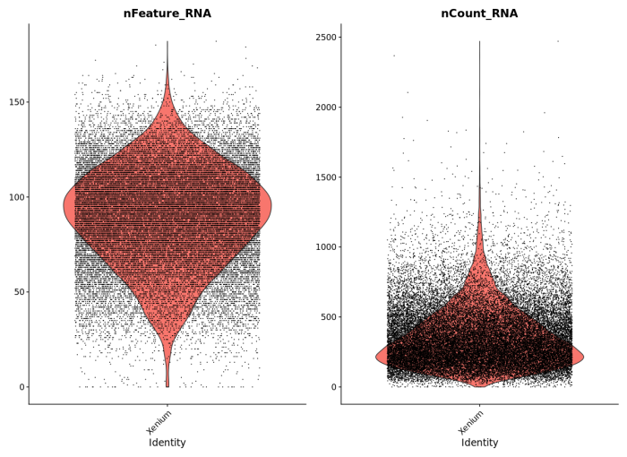
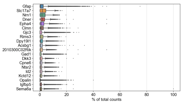
Likewise, we were able to follow this Scanpy tutorial and use the read_10x_mtx() function to load the matrix. The following plot shows the 20 genes that have the highest fraction of counts in each cell, across all cells, and it should be straightforward to proceed further with the tutorial and run the standard suite of single cell data analysis with this feature-cell matrix.
If you use Cellpose in your publication, please cite Cellpose based on citation guidelines here.