Note: 10x Genomics does not provide support for community-developed tools and makes no guarantees regarding their function or performance. Please contact tool developers with any questions. If you have feedback about Analysis Guides, please email analysis-guides@10xgenomics.com.
10x single cell technologies empower researchers to unravel the intricacies of biology with unprecedented precision, enabling them to explore biology at a resolution specific to individual cell types. There is a vast and ever-evolving landscape of community-developed tools available for annotating individual cell types. To help our customers explore the results of these tools in an approachable environment, we developed a software package, LoupeR, that can take single cell data in an R programming environment and convert it into a Loupe Browser file. This should make collaborations easier, especially between bioinformaticians and wet lab scientists.
In this tutorial, we use a Single Cell Gene Expression Flex dataset containing 157,323 cells isolated from 21 flash frozen human tissue samples from treated and untreated Non-Small Cell Lung Cancer (Lung Squamous Cell Carcinoma, LUSC) and Normal Adjacent (NADJ). The goal of this experiment is to identify lung cell types across squamous cell lung cancer disease states.
The goals of this Analysis Guide are to demonstrate:
- How to use a community tool, Azimuth, to generate cell type annotations in R.
- How to export those annotations in a format that can be imported into Loupe Browser.
- How to convert the Seurat object generated from Azimuth into a .cloupe file using LoupeR.
The code provided in this Analysis Guide was written in R version 4.2.1. The full session information, including the versions of various packages used, can be found at the bottom of this page.
Azimuth is an automated cell type annotation tool that uses a pre-annotated reference single cell dataset along with a feature-barcode matrix (the query dataset) as inputs. It compares the gene expression profile of each individual cell in the query dataset to the reference and its cell type assignments. This means that users need to choose an appropriate reference dataset, with annotations, to use this tool. The developers of Azimuth provide references for specific tissues through a database, which you may use if you do not have your own reference readily available. If you do not see your tissue of interest in Azimuth’s database, you may need to explore other cell type annotation tools that do not require a reference dataset. We recommend exploring several options before proceeding with any one tool, as each tool differs in its required inputs, algorithms, and accuracy, depending on your data. We have chosen to use Azimuth for this tutorial based on its ease of use, compatibility with R, and interoperability with 10x inputs. To learn about other cell type annotation tools, including those that do not require reference data, see our article: Web Resources for Cell Type Annotation.
Once Azimuth is run, a Seurat object is returned which contains:
- Cell annotations (at multiple levels of resolution, from broad cell type categories to more specific ones)
- Prediction scores (i.e. confidence scores) for each annotation
- Projection onto the reference-derived 2-dimensional UMAP visualization
- Mapping scores for the projection
Details and information about the Azimuth algorithm can be found in Stuart et al. 2019. Azimuth is compatible with a wide range of inputs, including Seurat objects, 10x HDF5 files, and Scanpy/h5ad files. Azimuth can be used in R, as demonstrated in this tutorial, or through a web app created by the developers. Simply click the "Go to App" button associated with the reference data that you would like to use on this page.
Azimuth is just one option among many for cell type annotation. To learn about other cell type annotation tools, including those that do not require reference data as input, see our article: Web Resources for Cell Type Annotation.
Next we will walk through the steps to generate cell type annotations and convert those data into a Loupe file. All files needed to execute the following script, including the R script itself, can be found in the compressed folder here: annotations-r-to-loupe.tar.gz. Be sure to upload all files into your working directory prior to beginning the tutorial. Note: the total time to completion for this tutorial, starting from installation on a laptop computer with 16 GB of memory, is around 2 hours.
Set your working directory to the directory containing the required files for this tutorial:
setwd(“/path/to/working/directory”)
Install and load remotes package (needed for installation of Azimuth):
install.packages("remotes")
library (remotes)
Install the remaining necessary packages:
install.packages("Seurat")
remotes::install_github("satijalab/azimuth", ref = "master")
install.packages("SeuratData")
Load the necessary libraries into your R environment:
library(Seurat)
library(Azimuth)
library(SeuratData)
Next, we install a reference dataset that will be used by Azimuth to generate annotations in our query dataset. The human lung tissue reference used for this tutorial is automatically downloaded as part of the SeuratData framework. More information about this reference can be found here.
#First view available datasets and double check the name of the reference we plan to use.
available_data<-AvailableData()
#Add a longer timeout option otherwise the download will fail
options(timeout = 1000)
#Install the human lung reference data
InstallData('lungref')
Next, read in the query data we plan to annotate:
data<- Read10X_h5("/path/to/working/directory/filtered_feature_bc_matrix.h5", use.names = TRUE, unique.features = TRUE)
And initialize a Seurat object of the data:
data<- CreateSeuratObject(data, project = "tutorial", assay = "RNA")
The RunAzimuth function takes the feature barcode matrix and Seurat object reference as inputs. This step takes about 45 min - 1 hr to complete on a 16 GB laptop.
Prediction<-RunAzimuth(data, "lungref")
Azimuth generates six total levels of annotation, from the broadest categories at level 1 to the most detailed categories at level 6 (named "finest level"). The level 3 annotations generated by Azimuth contain the level of detail needed to answer our research questions, but not so much detail that there is an overwhelming number of cell type categories, so we will focus on this level for downstream analysis.
If we take a closer look at the level 3 cell type categories, we can see that there is a “Rare” cell type population. The original paper that describes the lung reference and its annotations shows that this cell type category is actually a grouping of historically difficult-to-identify rare lung cell types, which include ionocytes, tuft cells, neuroendocrine cells, and certain immune cell subtypes (Sikkema, L., Ramírez-Suástegui, C., Strobl, D.C. et al., 2023).
Because Azimuth provides several levels of annotations ranging from broad to specific, we can see if these rare cells can, in fact, be assigned to more specific rare cell type categories using the finest level of annotation provided by Azimuth.
To do this, extract level 3 cell type annotations generated by Azimuth:
CellTypes_Azimuth<-Prediction@meta.data
CellTypes_Azimuth$Barcode<-rownames(CellTypes_Azimuth)
CellTypes_Azimuth$CustomLevel<-CellTypes_Azimuth$predicted.ann_level_3
Assign barcodes with "Rare" labels in level 3 to more specific ones using the finest level of annotations provided by Azimuth:
iix<-which(CellTypes_Azimuth$predicted.ann_level_3=="Rare")
CellTypes_Azimuth$CustomLevel[iix]<-CellTypes_Azimuth$predicted.ann_finest_level[iix]
Create output that can be added back into the Seurat object:
CellTypes_Azimuth<-CellTypes_Azimuth[,c("Barcode","CustomLevel")]
colnames(CellTypes_Azimuth)<-c("Barcode","CustomLevel")
Add cell type annotations to the Seurat object as metadata:
rownames(CellTypes_Azimuth)<-CellTypes_Azimuth$Barcode
Prediction[["CustomLevel"]]<-CellTypes_Azimuth$Barcode[match(rownames(Prediction@meta.data), CellTypes_Azimuth$CustomLevel)]
Prediction<-AddMetaData(object = Prediction, metadata = CellTypes_Azimuth$CustomLevel, col.name = "CellTypes")
Because we took data directly from the feature barcode matrix, we are missing some important metadata that would have otherwise been included after running cellranger aggr. To make sure that metadata is included in our final .cloupe file, we will add metadata about disease state groups to our Seurat object:
diseasestate <- read.csv("/path/to/working/directory/diseasestate.csv")
rownames(diseasestate) <- diseasestate$Barcode #need to import csv with disease state assignments by barcode
Prediction[["DiseaseState"]] <- diseasestate$Barcode[match(rownames(Prediction@meta.data), diseasestate$disease.state)]
Prediction <- AddMetaData(object = Prediction, metadata = diseasestate$disease.state, col.name = "DiseaseState")
Similarly, going from the feature barcode matrix to Loupe Browser will not allow us to include dimensionality reductions generated by Cell Ranger. Thus, we have to add the projections generated by the pipeline at this step. If you open the original .cloupe file for your analysis (automatically generated as an output of cellranger count/multi), then you can export these projections as a CSV and add them to the Seurat object. We have already saved these coordinates as a CSV in our working directory.
tSNE_coordinates <- read.csv("/path/to/working/directory/t-SNE-Projection.csv", stringsAsFactors = F, header = T, row.names = 1)
tSNE_coordinates_mat <- as(tSNE_coordinates, "matrix")
Prediction[['tSNE']] <- CreateDimReducObject(embeddings = tSNE_coordinates_mat, key = "tSNE_", global = T, assay = "RNA")
The last bit of metadata that we will add back in is the sample ID information so that we do not lose track of which cell barcode came from which sample:
sampleID <- read.csv("/path/to/working/directory/SampleID.csv", stringsAsFactors = F, header = T, row.names = 1)
sampleID$Barcode<- rownames(sampleID)
Prediction[["sampleID"]] <- sampleID$Barcode[match(rownames(Prediction@meta.data), sampleID$SampleID)]
Prediction <- AddMetaData(object = Prediction, metadata = sampleID$SampleID, col.name = "sampleID")
Install and load loupeR:
remotes::install_github("10XGenomics/loupeR")
library(loupeR)
loupeR::setup()
Run create_loupe_from_seurat command, which takes the Seurat object as input:
create_loupe_from_seurat(Prediction)
The command above will automatically generate a file named “converted.cloupe”. This file contains our original data, cell type assignments, experimental conditions, cellranger-generated t-SNE projections, and sample IDs.
If you would rather import the cell type assignments into an existing .cloupe file, you can save barcode and cell type assignment information as a CSV that can be imported into Loupe:
write.csv(CellTypes_Azimuth, "/path/to/working/directory/CellTypes_Azimuth.csv", row.names = FALSE)
The limitation of this approach is that you will not get all levels of annotation generated by Azimuth, only the ones you export one-by-one and add manually into Loupe.
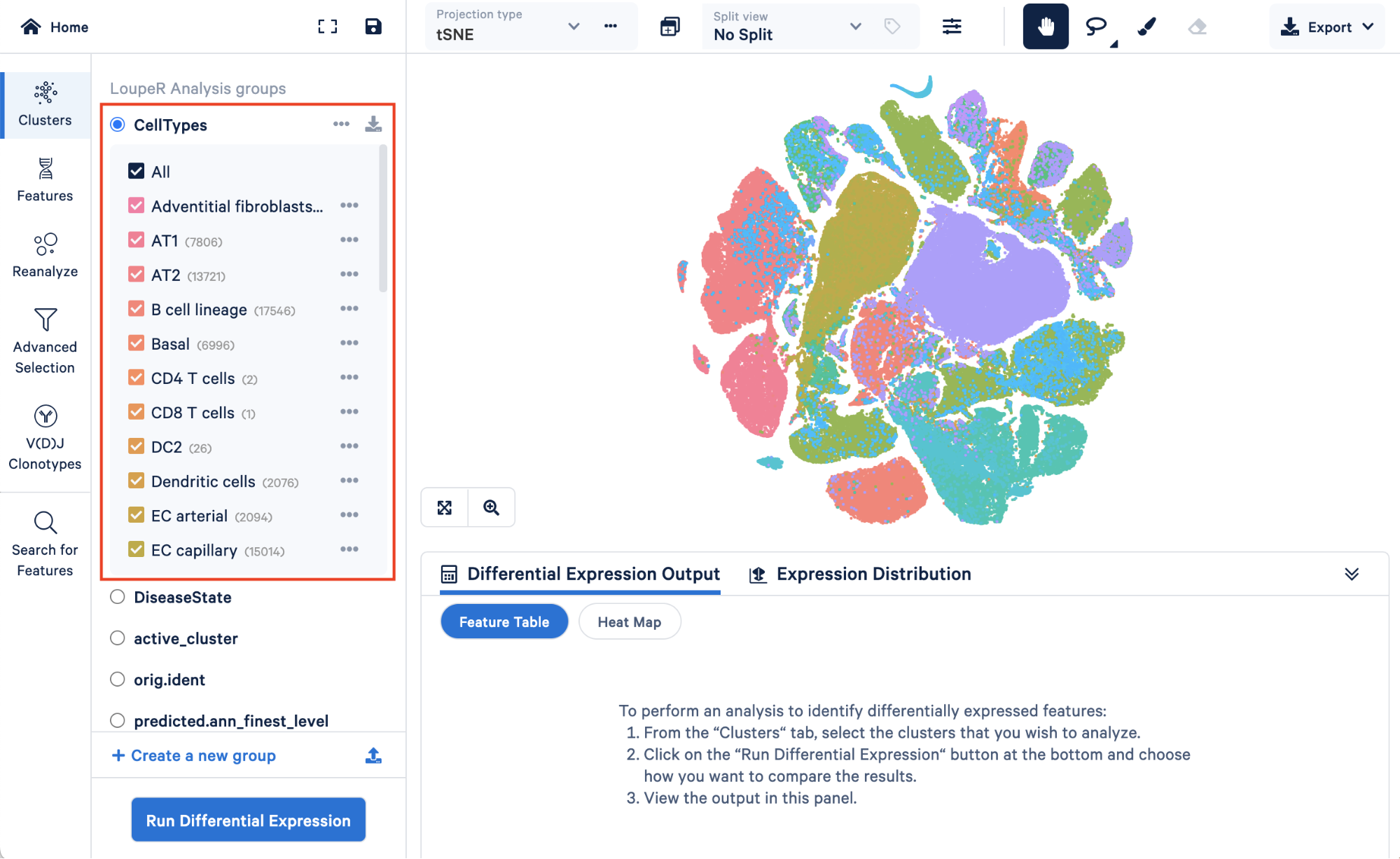
Opening your saved converted.cloupe file, you will first see the custom “CellTypes” annotations we generationed in Step 4 within “LoupeR Analysis groups”:
Below, we can see metadata that we added back in, “DiseaseState”, along with some groups that are automatically generated by Seurat, “active_cluster” and “orig.ident”.
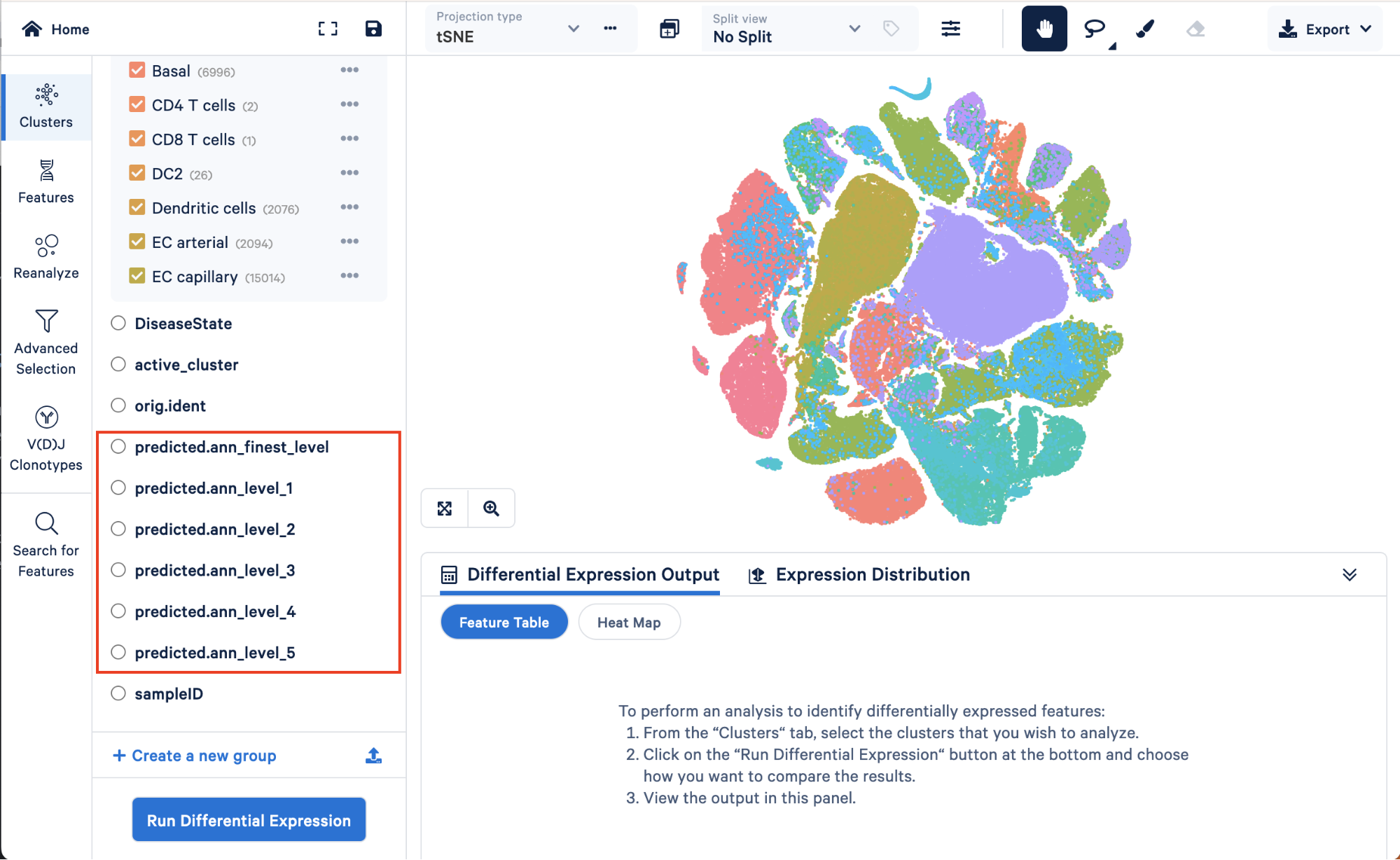
There are six levels of annotation, ranging from level 1 (the lowest resolution containing four cell types) to the finest level (containing 51 cell types):
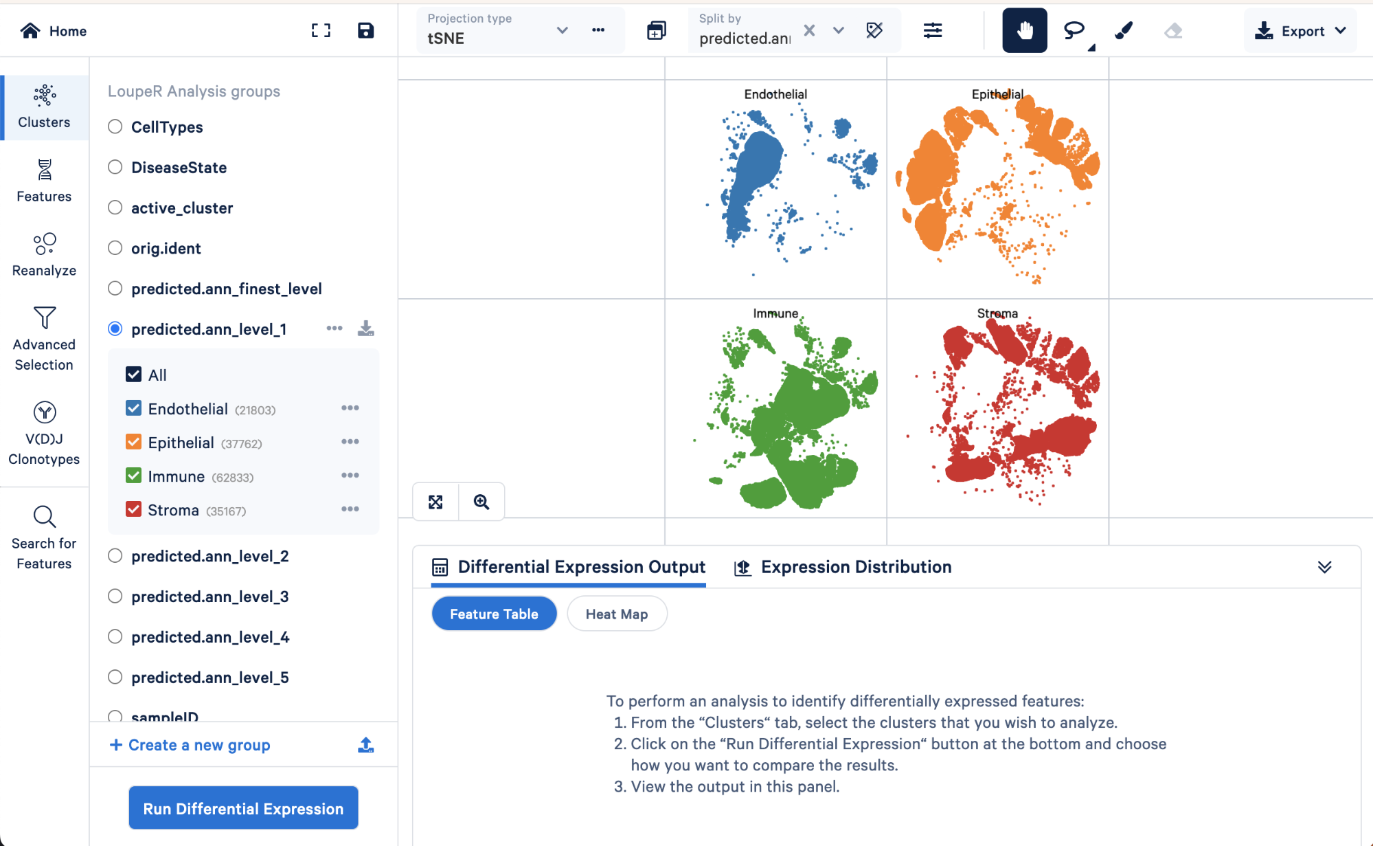
We can use the split view function in Loupe Browser to explore how the level 1 annotations relate to a finer level of annotation, level 3:
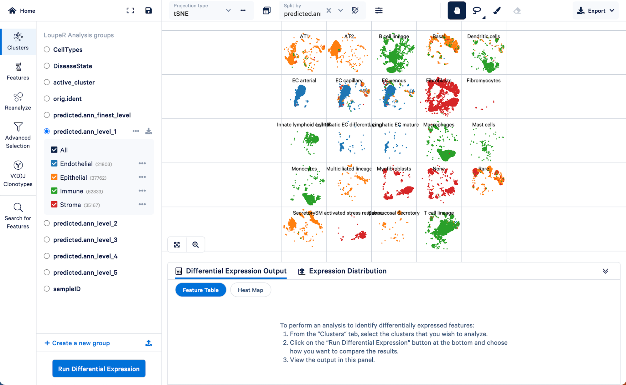
Here we can see the AT1 and AT2 (two major lung epithelial cell types), basal cells, multiciliated, secretory, rare, and submucosal secretory all primarily fall within the “Epithelial” assignment of level 1. Similarly, B cells, dendritic cells, innate lymphoid cells, macrophages, mast cells, monocytes, and T cell lineage cells all fall within the “Immune” cell type assignment of level 1. These results make sense biologically.
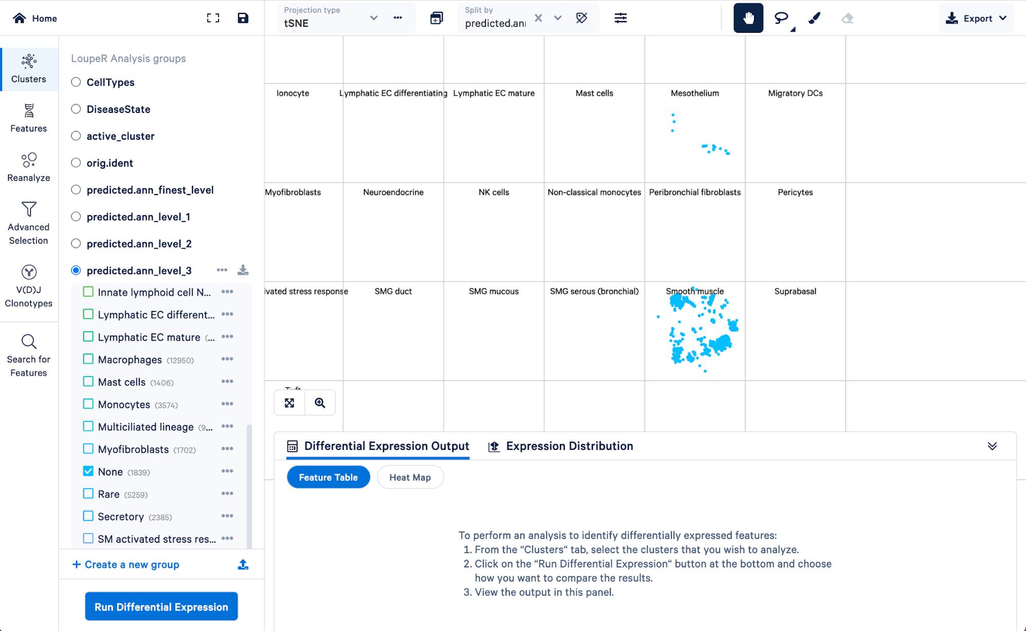
Note that there is a category called “None” in the level 3 annotation. These are cells that could not be given a confident assignment (probability score greater than 0.75) for one of the cell type categories in level 3. Using the finest level of annotation, we can see that cells in this category are mainly smooth muscle and mesothelial cells.
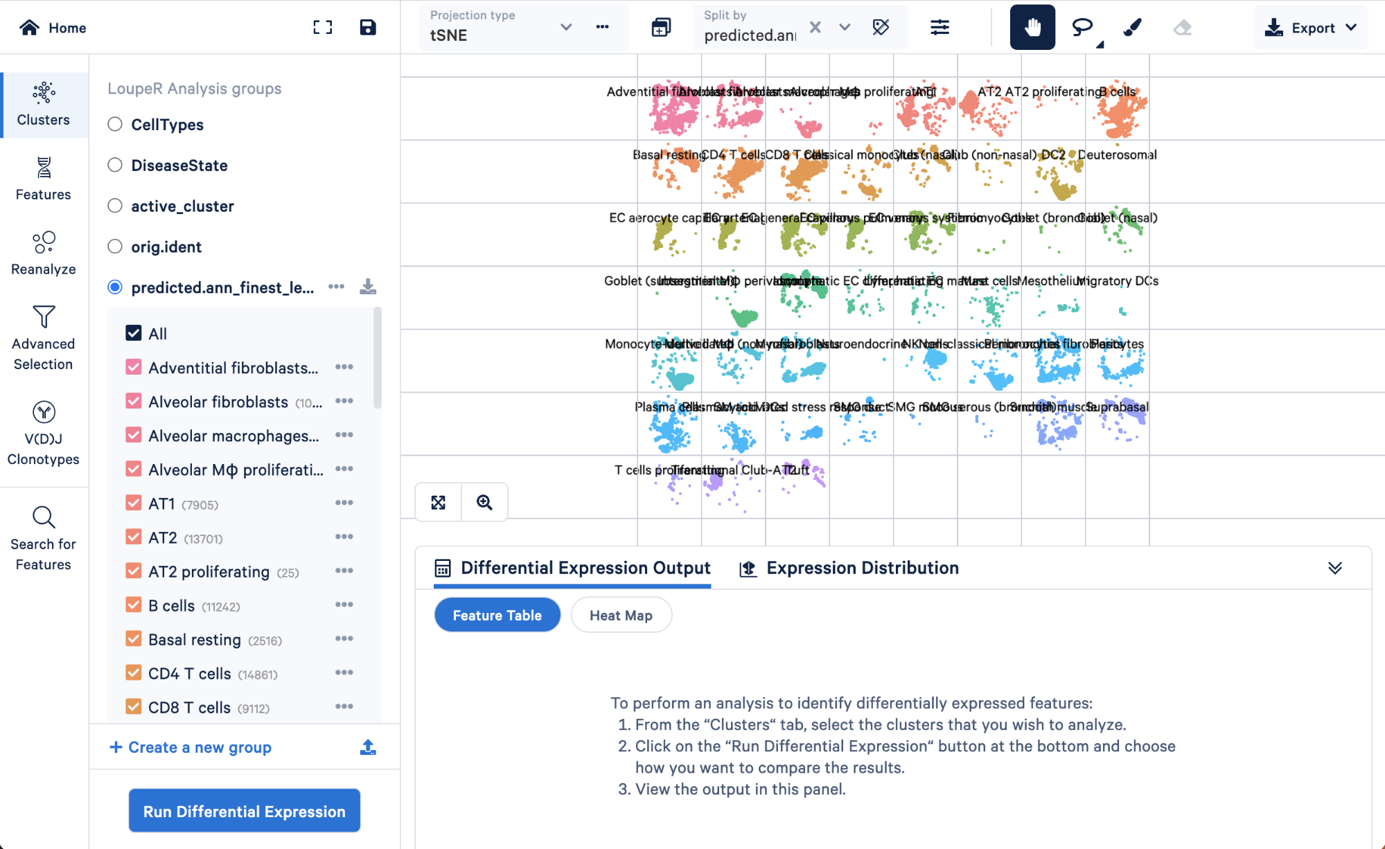
To visualize how cells in the “Rare” cell type group of the level 3 annotation were re-assigned in step 4, we can split those cells by the finest level.
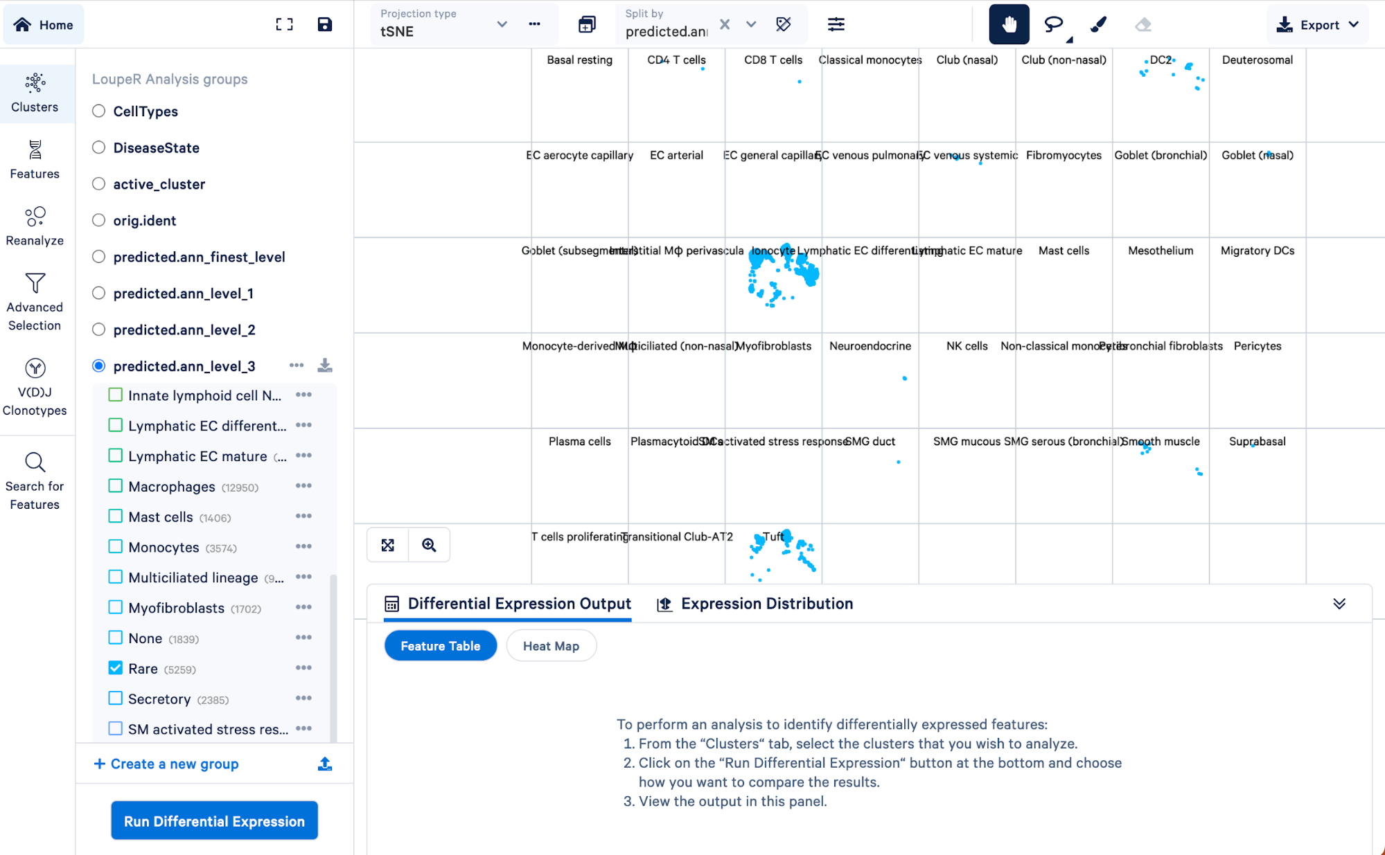
Doing this, we can see that the “Rare” cell type was mainly made up of ionocytes and tuft cells, with some DC2 cells, neuroendocrine, and smooth muscle cells. Level 3 did not have the resolution to capture these cell types, but we were able to take advantage of the multiple levels of annotation provided by Azimuth to uncover those rarer cell types.
In this Analysis Guide, we demonstrated how one can approach automated cell type annotation using a community-developed R tool, Azimuth. We showcased the utility of this particular tool by making use of the varying levels of annotation it provides, breaking up a non-descript, general cell type category into more specific rare cell subtypes. We then converted the annotated data in R into a .cloupe file using the new file conversion tool, loupeR. The resulting .cloupe file allows us to easily explore and navigate the results of Azimuth in 10x’s Loupe Browser software.
Now that we have generated our .cloupe file with Azimuth-generated annotations, we can use this file to ask interesting biological questions following our Single Cell Navigation Tutorial. The custom “CellTypes” generated here are the same ones featured in our Single Cell Navigation Tutorial where they are named “azimuth annotations”.
Watch our recorded webinar below for an introduction to Loupe Browser, Azimuth, and multi-sample comparisons followed by a live demonstration in Loupe Browser. The live demonstration begins at 19:04.
sessionInfo()
#R version 4.2.1 (2022-06-23)
#Platform: x86_64-conda-linux-gnu (64-bit)
#Running under: Amazon Linux 2
#Matrix products: default
#BLAS/LAPACK: /mnt/opt/R/R-4.2.1-#conda/env/lib/libopenblasp-r0.3.21.so
#locale:
# [1] LC_CTYPE=en_US.UTF-8 LC_NUMERIC=C LC_TIME=en_US.UTF-8 LC_COLLATE=en_US.UTF-8
# [5] LC_MONETARY=en_US.UTF-8 LC_MESSAGES=en_US.UTF-8 LC_PAPER=en_US.UTF-8 LC_NAME=C
# [9] LC_ADDRESS=C LC_TELEPHONE=C LC_MEASUREMENT=en_US.UTF-8 LC_IDENTIFICATION=C
#attached base packages:
#[1] stats graphics grDevices utils datasets methods base
#other attached packages:
#[1] loupeR_1.0.0 lungref.SeuratData_2.0.0 SeuratData_0.2.2 Azimuth_0.4.6
#[5] sp_1.5-0 SeuratObject_4.1.0 Seurat_4.1.1 shiny_1.7.2
#[9] shinyBS_0.61.1