This page describes the algorithms underlying the processing and analysis steps that occur on the Xenium Analyzer.
The Xenium workflow begins with sample preparation. Fresh frozen (FF) or formalin-fixed paraffin-embedded (FFPE) samples are mounted on Xenium slides. The samples are fixed and permeabilized (FF samples) or deparaffinized and decrosslinked (FFPE samples). Then, probe hybridization, ligation, and rolling circle amplification (RCA) are performed.
Once the sample has been prepared, imaging is performed in cycles on the Xenium Analyzer. During each cycle, fluorescently labeled probes for detecting RNA target sequences and other reagents, are automatically cycled in, imaged, and removed. The internal image sensor captures data across multiple Z-planes with a 0.75 μm step size across the entire tissue thickness for every field of view (FOV) in the user-selected region (see Region Selection Guidelines in the Xenium Analyzer instrument user guide). Image data are captured for multiple fluorescence channels in every cycle, which are processed and stitched to build a spatial map of the transcripts across the selected tissue section.
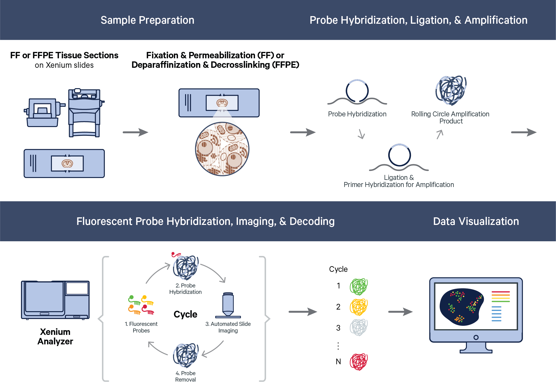
Thus, over the course of a run, the Xenium Analyzer’s internal image sensor collects 3D volumes across: 1) multiple FOVs, 2) multiple fluorescence channels, and 3) multiple cycles of chemistry and imaging. This produces terabytes of internal sensor data that are processed efficiently and analyzed across all cycle-channels to decode transcripts. Once transcripts are decoded, downstream analysis and visualization of Xenium raw data output — the spatial map of transcripts — can proceed.
The primary steps performed by the pipeline across cycles are:
- DAPI image processing: DAPI (Xenium Nuclei Staining Buffer) is a blue fluorescent DNA stain for visualizing nuclear DNA in fresh and fixed cells. In the Xenium workflow, DAPI staining is used to locate nuclei, inform cell segmentation, and produce a 3D tissue morphology image. DAPI images are captured once across all FOVs in the first cycle.
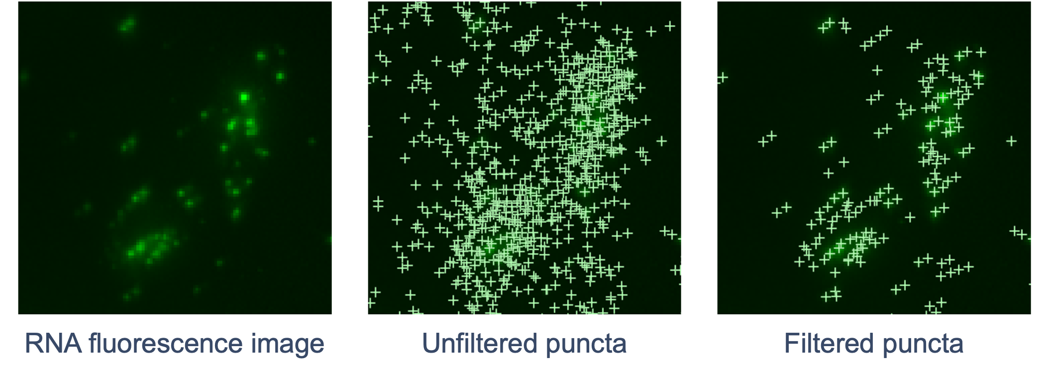
- RCA product image processing: For each cycle, images are captured in multiple color channels across all FOVs. Punctate fluorescent signals (puncta) are detected and filtered, and image distortion is corrected.
Cell segmentation occurs between cycles. DAPI images are used to infer cell boundaries using a machine learning algorithm.
The final steps of the pipeline include RCA product image registration, decoding, deduplication, secondary analysis, and generation of Xenium output data. Quality scores (Q-Scores) are estimated using controls for calibration (see Controls).
Image processing begins by mapping known physical features on the glass slide surface (fiducials) to set the image coordinate system. The instrument then identifies the upper bound of the tissue section to find the location of the first Z-slice. These pieces of information collectively determine the range of Z-slices to image. This process has been robust to all tested sections and tissue types.
The DAPI image process produces a complete 3D morphology image (the morphology.ome.tif output file) for each of the stained regions and determines the reference image volume that cells are segmented from and decoded transcripts are assigned to.
First, the lens distortion in internal sensor data is corrected. This is done computationally based on instrument calibration data, which are collected in order to characterize the optical system and are saved on-instrument. Next, the Z-stacks from internal sensor data (0.75 µm step size) are further subsampled to a 3 μm step size. This subsampling step size was determined empirically to be a useful resolution for cell segmentation quality.
Shared image features are then extracted from the regions where FOVs overlap. Feature matching is performed to estimate the offsets between adjoining FOVs. The offsets are used to ensure consistent alignment across the image (global alignment).
Finally, the 3D DAPI image volumes (Z-stacks) generated across FOVs are blended together to construct a stitched volume that is used for nucleus segmentation.
The goal of RCA product image processing is to detect and filter puncta and correct distortion. Performed for every channel and cycle, the 3D image volumes (Z-stacks) obtained for each FOV are processed to detect the puncta in 3D space that correspond to labeled RCA products. Images are currently captured in four color channels and 15 cycles (subject to change to accommodate platform growth). The RNA fluorescence image is scanned for punctum signals that stand out from the local background. The XYZ coordinates of each punctum are refined by examining local brightness. The signal intensity of the punctum is determined based on a fitted shape.
Next, the pipeline filters out puncta that are unlikely to be true transcripts (non-punctate or low quality signals). Similar to DAPI images, curvature distortion is corrected.
The goal of cell segmentation is to approximate boundaries between cells so that transcripts can be assigned to cells. Downstream, these results will be used to produce a cell-feature matrix, similar to those output by existing single cell and spatial technologies. It is possible to use third-party segmentation tools with the same morphology image that Xenium uses. Analysis Guides on this topic can be found on the 10x website. Xenium’s cell segmentation algorithm will evolve to accommodate platform growth - stay tuned!
The first step is to detect the locations of nuclei using the DAPI images and a custom neural network for nucleus segmentation. The neural network is trained on thousands of manually labeled image patches covering multiple tissue types. Any nucleus that has 95% or more of its pixel intensity lower than an intensity threshold of 100 photoelectrons will be removed.
Once the locations of nuclei in the sample have been identified by the model, a heuristic cell boundary expansion step is performed. The nucleus boundaries are expanded by 15 µm or until they encounter another cell boundary in X-Y. If cell boundaries overlap during expansion, they are resolved using an algorithm that is conceptually similar to Voronoi tessellation.
Xenium cell segmentation takes into account the 3D output from the DAPI image processing step for all Z-slices for better accuracy, but ultimately produces a flattened 2D segmentation mask for ease of use. The nuclear boundaries are consolidated to form non-overlapping 2D objects when projected in X-Y. Since the segmentation mask is 2D, transcripts are assigned to 2D shapes based on their X and Y coordinates.
Nucleus and cell boundary polygons are also provided in the outputs. They are approximations of the segmentation masks and are used for efficient visualization of nucleus and cell segmentation in Xenium Explorer and other analysis software.
For each FOV, puncta across channels and cycles must be aligned to reduce differences in image offset, rotation, and magnification. This is important for accurate transcript decoding. The localized puncta from each channel and cycle are registered so that puncta corresponding to the same original RNA molecule are aligned tightly in 3D. Nonlinear transformations are fitted such that all the puncta are aligned to the reference morphology image.
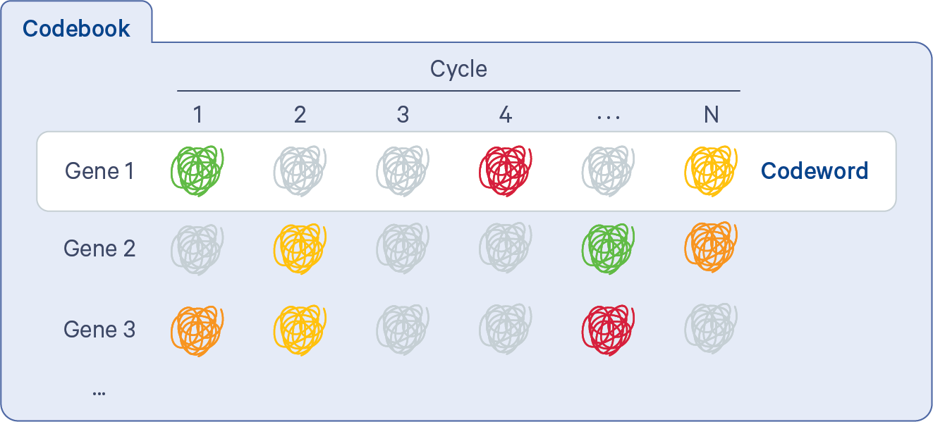
In order to proceed from puncta to transcripts, decoding must be performed. The Xenium codebook contains a collection of codewords that are assigned to genes in a given gene panel. The pipeline uses the gene_panel.json to specify a given gene name to an indexed codeword. Each codeword is defined based on a pattern of fluorescent signal intensities recorded across channels and cycles (see diagram below). Some codewords are reserved for negative controls.
When selecting the codeword assigned to each gene, the Xenium panel design process attempts to keep the predicted transcript density in each cycle-channel in each known cell type as uniform as possible, using single cell reference cell type data. In particular, high expression genes that are coexpressed in the same cell type will be assigned codewords in different cycle-channels as much as possible (more details on the Getting Started with Xenium Panels page).
The fluorescent signals from all channels and cycles are compared to the codebook using a global (across all FOVs) maximum likelihood approach based on probabilistic modeling. The decoding process itself does not make per cycle-channel calls. Instead, it assigns probabilities to each possible codeword given all of the information at a spatial location and chooses the most probable. This approach considers attributes such as puncta location, their color and cycle of detections, and signal intensities. Each transcript is imaged in a bright state five times across 60 cycle-channels (15 cycles x 4 channels).
The cell-feature matrix and Xenium Analyzer’s secondary analyses only include transcripts with a Q-Score ≥ 20. Final Q-Scores are reported in the transcript data output files.
A Phred-style calibrated quality score is assigned to each decoded transcript to signify the confidence in the decoded transcript identity. The quality score is derived from the likelihood of the maximum likelihood codeword (i.e., the codeword that best explains the observed data), compared to the likelihood of other sub-optimal codewords. This yields a raw Q-Score. Codewords are then mapped to targets using the gene panel information.
Final Q-Scores are obtained first by putting the full range of raw Q-Scores into bins. Then, the raw Q-Scores in each bin are calibrated by the proportion of "Negative Control Codewords" in the bin. A final Q-Score is assigned to each raw Q-Score bin, to ensure that Q-Scores in each bin are correctly calibrated. Control codewords are built into the process to ensure that the final Q-Scores are accurately calibrated.
- Negative control codewords are codewords in the codebook that do not have any probes matching that code. They are chosen to meet the same requirements as regular codewords and can be used to assess the specificity of the decoding algorithm.
- Negative control probes are probes that exist in the panels but target non-biological sequences. They can be used to assess the specificity of the assay.
- Unassigned codewords are unused codewords. There is no probe in a particular gene panel that will generate the codeword.
- The Deprecated codewords category is assigned to codewords that are not used in the Xenium Onboard Analysis pipeline.
After decoding, the results are combined from all FOVs. Duplicate decoded transcripts in overlapping regions between adjoining FOVs are reconciled into one transcript, based on a nearest neighbor analysis that considers transcript identity and Q-Score. The deduplicated transcripts are assigned global coordinates based on the reference morphology image obtained from the DAPI image processing step (morphology.ome.tif).
Decoded and deduplicated transcripts in 3D with Q-Scores ≥ 20 are assigned to directly overlapping segmented cells to produce a cell-feature matrix. This matrix can be analyzed using conventional and novel single cell and spatial analysis approaches, facilitating integration with existing single cell and spatial datasets.
Xenium’s onboard analysis uses the same algorithms as Cell Ranger for single cell gene expression for performing secondary analysis on the cell-feature matrix (PCA, UMAP, graph-based clustering, differential expression analysis). t-SNE projection is not supported in Xenium onboard analysis.