Note: 10x Genomics does not provide support for community-developed tools and makes no guarantees regarding their function or performance. Please contact tool developers with any questions. If you have feedback about Analysis Guides, please email analysis-guides@10xgenomics.com.
10x Genomics single cell assays normally produce a low level of background RNA counts. One source is from cell-free RNA molecules in the cell suspension (ambient mRNA) which can lead to inflated UMI counts, even in cell-free GEMs. Ambient mRNA could derive from ruptured, dead or dying cells, or from other exogenous sources of contamination. If not accounted for, and especially if present at moderate to high levels, background UMI counts could lead to systematic biases or batch effects in downstream analyses (Fleming et al.).
High background counts tend to occur more frequently in certain tissue types (Madisson et al), particularly when working with single cell nuclei samples. The nuclei preparation protocols typically release cytoplasmic RNA into solution (please see our nuclei isolation product). The barcode rank plot may not have a steep cliff, due to increased background RNA. However such data are still usable even without background subtraction.
To computationally identify and remove ambient RNA, specifically in the nuclei datasets, one can make use of community-developed tools. In this article, we will use the remove-background algorithm (Fleming et al.) implemented in the CellBender python package. CellBender uses a machine learning model that is used to train the background RNA profile, distinguish cell-containing droplets from empty ones, and retrieve cleaner gene expression profiles. We then switch from python to R to further explore clustering downstream in Seurat.
This article assumes the raw sequence data have already been demultiplexed using either the bcl2fastq or mkfastq pipelines (i.e., you are starting with FASTQ files). Also you must run the cellranger count or multi pipelines for alignment and annotation of reads, barcode error correction, and generation of feature barcode matrices.
All the steps in CellBender are in python. If you don't have python in your system yet, please install python. You may also consider running python using any IDE. If you do not have a conda environment, you could try miniconda.
The softwares used in this article can be run on a Linux server. Software versions used in this article include:
- Python v3.8
- CellBender v0.2.0
- R version v4.0
- Seurat v4
Create a conda environment and activate it. We use python 3.8 to suit our system environment.
conda create -n CellBender python=3.8
source activate CellBender
Install the prerequisite modules and CellBender following the instructions here. The CellBender version used in this article is v0.2.0.
This section uses commands found in this CellBender tutorial. Please activate the CellBender environment if you are starting from this section.
Load the raw feature barcode matrix file from your cellranger output using the command below.
cellbender remove-background \
--input raw_feature_bc_matrix.h5 \
--output output.h5 \
--expected-cells (value) \
--total-droplets-included (value) \
--fpr 0.01 \
--epochs 150
What do the CellBender parameters listed above mean?
remove-background: This is a module within the CellBender package. It implements a fast and scalable maximum-likelihood (ML) inference algorithm that inputs raw gene-by-cell count matrices and UMI information along with certain parameters. It then filters any ambient RNA (and barcode-swapped reads) from the count matrix, producing a new count matrix and determining which barcodes contain real cells.
--expected-cells: This corresponds to the expected recovered/targeted cells for your experimental design. Choose the number that you targeted. One way to estimate this is using the cells metric found in the web_summary.html file output by Cell Ranger. For the good and compromised datasets used in this tutorial, we used 10k and 5k cells respectively.
--total-droplets-included: Choose a number that extends a few thousand barcodes into the “empty droplet plateau”. See the UMI curve below (Fig. 1, ref), where an appropriate initial choice would be 15,000 or 20,000. However, this varies with the degree of noise in the dataset. Every droplet to the right of this number on the UMI curve should be nearly empty. This kind of UMI curve can be seen in the websummary.html output from cellranger count (Fig. 2, technote). Try including some droplets that you think are empty. But be aware that the _larger this number, the longer the algorithm takes to run. In this tutorial, we use 30,000.
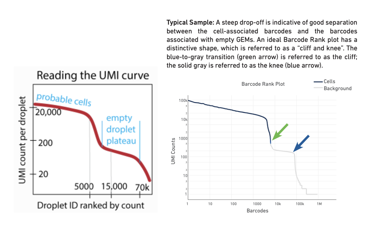
Left: Reading the UMI curve (note the transition region is the region we are interested in CellBender) Right: Typical barcode rank plot from Cell Ranger web summary
--fpr: The default value is 0.01. You can generate a few output count matrices by choosing a few values such as 0.01 0.05, 0.1, 0.3 and compare the downstream results (by visualizing clusters and cell type annotation results, more details in later sections). In this tutorial, we used default (0.01) for the good dataset, and used 0.3 for the compromised dataset.
--epochs: epochs is the number of complete passes through a training dataset used in Machine Learning algorithms. The number of epochs can be set to an integer value between one and infinity. For single cell GEX datasets, 150 is typically a good starting choice (ref).
All other optional arguments are discussed here.
Results & Discussion
Datasets used: For this tutorial, we will use a good PBMC dataset and a compromised dataset. You could also use any of your own dataset(s) to follow this tutorial.
PBMC 10k
The clean PBMC 10k v3 dataset can be downloaded here or by using the command line below:
wget https://cf.10xgenomics.com/samples/cell-exp/6.1.2/10k_PBMC_3p_nextgem_Chromium_X/10k_PBMC_3p_nextgem_Chromium_X_raw_feature_bc_matrix.h5
For this dataset, the command below was used to run CellBender. Runtime for this PBMC 10k dataset on a local server with 12 cores and 96 GB RAM takes about five hours. If you have a CUDA GPU, you may consider --cuda mode for a faster analysis time.
cellbender remove-background \
--input 10k_PBMC_3p_nextgem_Chromium_X_raw_feature_bc_matrix.h5 \
--output output.h5 \
--expected-cells 10000 \
--total-droplets-included 30000 \
--fpr 0.01 \
--epochs 150
After running CellBender on this 10K dataset, one of the outputs we obtain is a PDF that shows the below rank-ordered total UMI plot which has cells that are in the transition region.
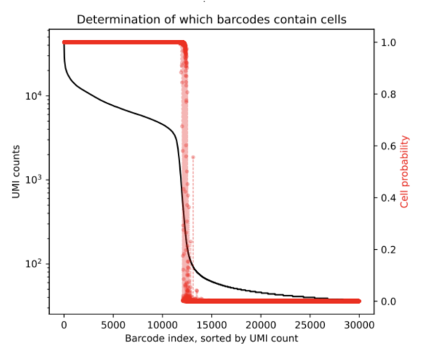
From the resulting cell_barcodes.csv file, we can ascertain that the ambigious region was found to contain an additional 272 cells. This is a clean dataset and we do not expect a lot of background. CellBender generates a new filtered count matrix determining which barcodes contain cells which can be used for further downstream analysis. All output files from a CellBender run are explained here.
A compromised nuclei dataset
For a not-so-clean dataset, after a couple of iterations, the below parameters were used to run CellBender.
cellbender remove-background \
--input raw_feature_bc_matrix.h5 \
--output output.h5 \
--expected-cells 5000 \
--total-droplets-included 30000 \
--fpr 0.3 \
--epochs 150
After running CellBender on this nuclei dataset we obtain the below rank-ordered total UMI plot that shows the cells that are in the transition region.
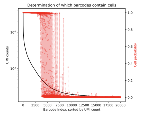
From the results, we can ascertain that the ambigious region was found to contain an additional 1,430 cells (based on the resulting cell_barcodes.csv file). This mockup dataset had a high background level and so we expect more cells to be returned by the remove-background analysis pipeline. CellBender generates a new filtered count matrix determining which barcodes contain cells which can be used for further downstream analysis. All output files from a CellBender run are explained here.
Downstream Analysis: Clustering & Cell Type Annotation
After cleaning up the data with CellBender, you might be interested in doing additional downstream analysis, such as clustering and cell type annotation (see also web resources on cell type annotation methods). You may also consider applying any quality control filters directly on the count matrices generated by CellBender before any downstream analysis.
In this article, we will take the analysis journey a bit further to illustrate how you can implement clustering analysis on CellBender's output using Seurat's Guided clustering tutorial in R. This analysis was performed on the compromised nuclei dataset. The filtered feature barcode matrix from CellBender's remove-background pipeline is used as the input for this analysis. The cell type annotations were performed using custom methods and you may consider using annotation methods that works best for your datasets. Shown below are the UMAP and cell type annotation results using the output from Cell Ranger and CellBender respectively.
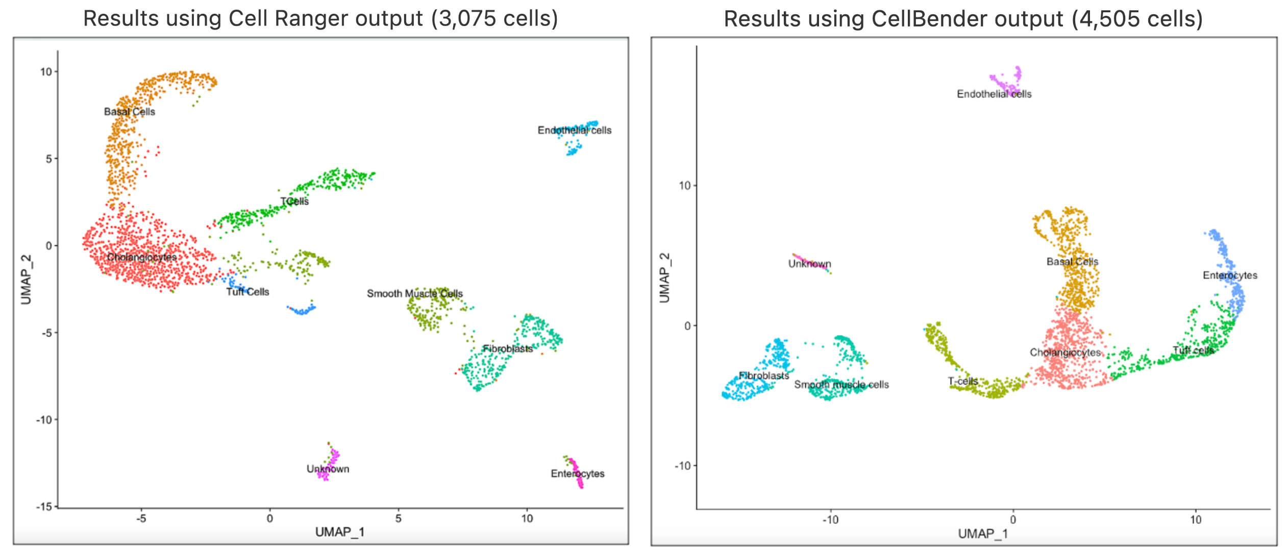
In our analyses, we found that the same clusters were obtained using the same value for the R code in Seurat’s FindClusters parameter. Both runs returned same cell types, which indicates that using Cell Ranger results directly are appropriate for this case. The full session info is available via the code template below.
# ----------------------------------------------------------------------------------------------------
# Disclaimer: The code block below is for illustrations only.
# It has been referenced from various resources and modified for the dataset used for this article.
# 10x Genomics does not support or guarantee third-party tools.
======================================================================================================
####################
# Install packages #
####################
install.packages('remotes')
remotes::install_version(package = 'Seurat', version = package_version('x.y.z'))
library(Matrix)
library(Seurat)
# ----------------------------------------------------------------------------------------------------------
# The below library is for CellBender output version compatibility with the current version of Seurat v4 Tutorial.
# Please find the issue commit here (https://github.com/broadinstitute/CellBender/issues/57)
# This may or may not be applicable to CellBender versions above v0.2.0
# ============================================================================================================
ReadCB_h5 <- function(filename, use.names = TRUE, unique.features = TRUE) {
if (!requireNamespace('hdf5r', quietly = TRUE)) {
stop("Please install hdf5r to read HDF5 files")
}
if (!file.exists(filename)) {
stop("File not found")
}
infile <- hdf5r::H5File$new(filename = filename, mode = 'r')
genomes <- names(x = infile)
output <- list()
if (hdf5r::existsGroup(infile, 'matrix')) {
# cellranger version 3
message('CellRanger version 3+ format H5')
if (use.names) {
feature_slot <- 'features/name'
} else {
feature_slot <- 'features/id'
}
} else {
message('CellRanger version 2 format H5')
if (use.names) {
feature_slot <- 'gene_names'
} else {
feature_slot <- 'genes'
}
}
for (genome in genomes) {
counts <- infile[[paste0(genome, '/data')]]
indices <- infile[[paste0(genome, '/indices')]]
indptr <- infile[[paste0(genome, '/indptr')]]
shp <- infile[[paste0(genome, '/shape')]]
features <- infile[[paste0(genome, '/', feature_slot)]][]
barcodes <- infile[[paste0(genome, '/barcodes')]]
sparse.mat <- sparseMatrix(
i = indices[] + 1,
p = indptr[],
x = as.numeric(x = counts[]),
dims = shp[],
giveCsparse = FALSE
)
if (unique.features) {
features <- make.unique(names = features)
}
rownames(x = sparse.mat) <- features
colnames(x = sparse.mat) <- barcodes[]
sparse.mat <- as(object = sparse.mat, Class = 'dgCMatrix')
# Split v3 multimodal
if (infile$exists(name = paste0(genome, '/features'))) {
types <- infile[[paste0(genome, '/features/feature_type')]][]
types.unique <- unique(x = types)
if (length(x = types.unique) > 1) {
message("Genome ", genome, " has multiple modalities, returning a list of matrices for this genome")
sparse.mat <- sapply(
X = types.unique,
FUN = function(x) {
return(sparse.mat[which(x = types == x), ])
},
simplify = FALSE,
USE.NAMES = TRUE
)
}
}
output[[genome]] <- sparse.mat
}
infile$close_all()
if (length(x = output) == 1) {
return(output[[genome]])
} else{
return(output)
}
}
# --------------------------------------------------------------------------------------------------------
# Below is an example template for running clustering analysis based on Seurat Guided clustering tutorial.
# You may consider fine tuning the parameters specific for your datasets.
# ==========================================================================================================
file <- "/Users/nisha.pillai/Documents/cbfirstrun_filtered.h5"
data <- ReadCB_h5(filename = file, use.names = TRUE)
obj <- CreateSeuratObject(counts = data, min.cells = 3, min.features = 200)
VlnPlot(obj, features = c("nFeature_RNA", "nCount_RNA"), ncol = 2)
cbres <- NormalizeData(obj)
cbres <- FindVariableFeatures(cbres, selection.method = "vst", nfeatures = 2000)
cbres <- ScaleData(cbres)
cbres <- FindVariableFeatures(cbres)
cbres = RunPCA(cbres)
cbres <- FindNeighbors(cbres, dims = 1:10)
cbres <- FindClusters(cbres, resolution = 0.5)
cbres <- RunUMAP(cbres, dims = 1:9)
DimPlot(cbres, reduction = "umap")
#cbres <- FindNeighbors(cbres, k.param = 50)
# ---------------------------------------------------------------------------------------------------------
# Differentially expressed genes for the first cluster.
# You may loop this for remaining clusters to find the top significant genes for cell annotation purposes.
# ===========================================================================================================
cluster0.markers <- FindMarkers(cbres, ident.1 = 0, min.pct = 0.25, only.pos = TRUE)
# ----------------------------------------------------------------------------------------------------
# The below annotations is based on the the top significant genes per cluster.
# For the compromised dataset, the annotations were generated using custom methods.
# You may consider using any cell type annotation method of your choice for your specific projects.
# The below rename of cluster ids works for the compromised dataset that had returned 9 clusters in UMAP;
# Please customize the renaming of cluster ids according to the UMAP clusters & annotations specific for your data.
# =====================================================================================================
new.cluster.ids <- c("Cholangiocytes", "Basal Cells", "T-cells", "Tuft cells", "Smooth muscle cells", "Fibroblasts", "Enterocytes", "Endothelial cells", "Unknown")
names(new.cluster.ids) <- levels(cbres)
cbres <- RenameIdents(cbres, new.cluster.ids)
DimPlot(cbres, reduction = "umap", label = TRUE, pt.size = 0.5) + NoLegend()
# -----------------------------------------------
# session info used for the clustering analysis
# ===============================================
print(sessionInfo())
R version 4.0.2 (2020-06-22)
Platform: x86_64-apple-darwin17.0 (64-bit)
Running under: macOS 10.16
Matrix products: default
LAPACK: /Library/Frameworks/R.framework/Versions/4.0/Resources/lib/libRlapack.dylib
locale:
[1] en_US.UTF-8/en_US.UTF-8/en_US.UTF-8/C/en_US.UTF-8/en_US.UTF-8
attached base packages:
[1] stats graphics grDevices utils datasets methods base
other attached packages:
[1] sp_1.5-0 SeuratObject_4.1.0 Seurat_4.1.1 Matrix_1.4-1
In conclusion, cellbender remove-background recovers more cells, many of which lie further down the UMI curve. To verify if these cells cluster together with the other cell calls, a clustering analysis can be performed. Either the filtered matrix h5 file generated from a CellBender run can be used in third party tools like Seurat as illustrated above, or one can provide the cell barcodes CSV file from a CellBender run as an argument to cellranger reanalyze pipeline to visualise the clustering results on Loupe Browser.