Note: 10x Genomics does not provide support for community-developed tools and makes no guarantees regarding their function or performance. Please contact tool developers with any questions. If you have feedback about Analysis Guides, please email analysis-guides@10xgenomics.com.
Variation in different Chromium Single Cell ATAC (Assay for Transposase Accessible Chromatin) samples can be affected by technical factors, such as laboratory conditions or reagent choices. These batch effects may confound true biological variation between samples. Therefore, correcting the batch effects can be useful for data analysis.
If you are combining libraries generated by Chromium Single Cell ATAC v1.1 and v2 reagents, you might observe systematic differences in chromatin structure profiles between libraries. Here, we will demonstrate how to use community-developed tools to merge and correct batch effects between Single Cell ATAC v1.1 and v2 data. The same procedure could also be used to correct other types of batch effects.
In this tutorial, we will use the Harmony batch effect correction algorithm (Korsunsky et al. 2019) implemented in the Signac R package. The Harmony algorithm is available on GitHub, and Signac has tutorials for integration.
cellranger-atac aggr pipeline also has a chemistry batch correction feature, which was only designed to correct for systematic variability in chromatin accessibility caused by different versions of the Chromium Single Cell ATAC chemistries. The method described in this tutorial can also be used to correct for chemistry batch effects, as well as other types of batch effects.All the steps in this tutorial are written in R. If you do not have R installed yet, first install R. We also recommend running R in RStudio.
First, run these commands to install the libraries:
install.packages("dplyr") install.packages("Seurat") install.packages("harmony") install.packages("Signac") install.packages("hdf5r") install.packages("BiocManager") BiocManager::install("GenomicRanges") BiocManager::install("Rsamtools")
Then load these libraries:
library(dplyr) library(Seurat) library(harmony) library(Signac) library(GenomicRanges)
Set a random seed:
set.seed(1234)
The two datasets used in this tutorial can be found here: dataset 1: 10k Human PBMCs, ATAC v1.1 cells and dataset 2: 10k Human PBMCs, ATAC v2 cells.
Use the download.file function in R to download the matrix H5 files.
# Set working directory before downloading files setwd(".") # Download dataset 1 filtered_peak_bc_matrix.h5 file download.file("https://cf.10xgenomics.com/samples/cell-atac/2.1.0/10k_pbmc_ATACv1p1_nextgem_Chromium_X/10k_pbmc_ATACv1p1_nextgem_Chromium_X_filtered_peak_bc_matrix.h5","10k_pbmc_ATACv1p1_nextgem_Chromium_X_filtered_peak_bc_matrix.h5") # Download dataset 2 filtered_peak_bc_matrix.h5 file download.file("https://cf.10xgenomics.com/samples/cell-atac/2.1.0/10k_pbmc_ATACv2_nextgem_Chromium_X/10k_pbmc_ATACv2_nextgem_Chromium_X_filtered_peak_bc_matrix.h5","10k_pbmc_ATACv2_nextgem_Chromium_X_filtered_peak_bc_matrix.h5")
If you have your own dataset to analyze, the filtered_peak_bc_matrix.h5 file is located at the outs directory of cellranger-atac count.
This section uses commands found in the Signac tutorial. It creates two Seurat objects. The Signac tool has a function called "Read10X_h5" that will automatically take h5 file from Cell Ranger ATAC and input them into the R environment.
# load the filered peak barcode matrix for each object # If using your own data, please specify the full path, for example: "/Users/mickey.mouse/Documents/mydata/outs/filtered_peak_bc_matrix.h5" counts.10k_v1p1 <- Read10X_h5("10k_pbmc_ATACv1p1_nextgem_Chromium_X_filtered_peak_bc_matrix.h5") counts.10k_v2 <- Read10X_h5("10k_pbmc_ATACv2_nextgem_Chromium_X_filtered_peak_bc_matrix.h5") # create objects pbmcv1p1_assay <- CreateChromatinAssay(counts = counts.10k_v1p1, sep = c(":", "-")) pbmcv1p1 <- CreateSeuratObject(pbmcv1p1_assay, assay = "peaks") pbmcv2_assay <- CreateChromatinAssay(counts = counts.10k_v2, sep = c(":", "-")) pbmcv2 <- CreateSeuratObject(pbmcv2_assay, assay = "peaks") # add information to identify datasets of origin pbmcv1p1$dataset <- 'pbmcv1p1' pbmcv2$dataset <- 'pbmcv2' # view the information of the objects: pbmcv1p1 pbmcv2
The output of pbmcv1p1 and pbmcv2 objects should be similar to the following:
An object of class Seurat 113692 features across 10609 samples within 1 assay Active assay: peaks (113692 features, 0 variable features) An object of class Seurat 164487 features across 10273 samples within 1 assay Active assay: peaks (164487 features, 0 variable features)
Use the merge function to combine the objects without batch correction, and visualize them using the head and tail functions.
unintegrated <- merge(x = pbmcv1p1, y = pbmcv2, add.cell.ids = c("pbmcv1p1", "pbmcv2")) # view the head of the combined objects head(colnames(unintegrated))
The output of head(colnames(unintegrated)) should be like the following:
"pbmcv1p1_AAACGAAAGAACGCCA-1" "pbmcv1p1_AAACGAAAGACAGCTG-1" "pbmcv1p1_AAACGAAAGAGTAAGG-1" "pbmcv1p1_AAACGAAAGATGCGCA-1" "pbmcv1p1_AAACGAAAGGCAGATC-1" "pbmcv1p1_AAACGAAAGTCATACC-1"
Next, we visualize the data before batch correction.
# Standard pre-processing steps before visualization # Compute the term-frequency inverse-document-frequency normalization on a matrix used in LSA (Latent semantic analysis) unintegrated <- RunTFIDF(unintegrated) # Find most frequently observed features unintegrated <- FindTopFeatures(unintegrated, min.cutoff = 20) # Run singular value decomposition, finds a few approximate largest (or, optionally, smallest) singular values and corresponding singular vectors of a sparse or dense matrix unintegrated <- RunSVD(unintegrated) # Runs the Uniform Manifold Approximation and Projection (UMAP) dimensional reduction technique unintegrated <- RunUMAP(unintegrated, dims = 2:50, reduction = 'lsi') # Dimensional reduction plot DimPlot(unintegrated, group.by = 'dataset', pt.size = 0.1)
More details on the functions and parameters can be found in the Signac tutorial. This tutorial used the default settings.
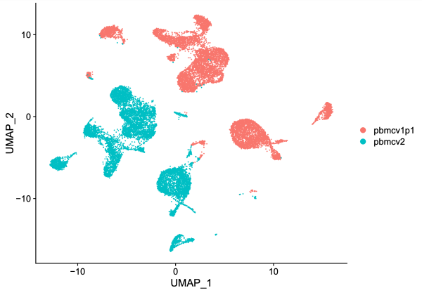
On the UMAP plot above, cells from dataset 1 (10k Human PBMCs, ATAC v1.1; red) are separated from cells from dataset 2 (10k Human PBMCs, ATAC v2; blue). Given that these are both human PMBCs, one might expect better overlap between the two samples. We suspect that chemistry batch effects could cause the lack of overlap.
In this step, use Harmony to correct the batch effects between the two samples.
hm.integrated <- RunHarmony(object = unintegrated, group.by.vars = 'dataset', reduction = 'lsi', assay.use = 'peaks', project.dim = FALSE) hm.integrated <- RunUMAP(hm.integrated, dims = 2:30, reduction = 'harmony') DimPlot(hm.integrated, group.by = 'dataset', pt.size = 0.1)
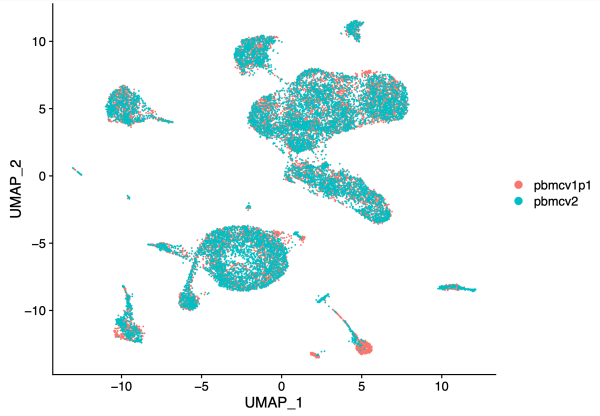
After batch correction in Harmony, note that the two PBMC samples largely overlap.
Next, we want to export the corrected UMAP projections to a CSV file that can be loaded into Loupe Browser. Some of the code was adapted from "How to export UMAP data for 10X Loupe Cell Browser?" tutorial.
# split the object corrected.data <- SplitObject(hm.integrated, split.by = "dataset") # edit the barcodes into a format that is compatible with the Loupe Browser pbmcv1p1.barcode <- rownames(Embeddings(object = corrected.data$pbmcv1p1, reduction = "umap")) pbmcv1p1.barcode <- gsub("pbmcv1p1_","",pbmcv1p1.barcode) pbmcv1p1.barcode <- gsub('.{2}$','',pbmcv1p1.barcode) pbmcv1p1.barcode <- paste(pbmcv1p1.barcode,"-1", sep="") pbmcv1p1.proj <- Embeddings(object = corrected.data$pbmcv1p1, reduction = "umap") UMAP.pbmcv1p1 <- cbind("Barcode" = pbmcv1p1.barcode, pbmcv1p1.proj) pbmcv2.barcode <- rownames(Embeddings(object = corrected.data$pbmcv2, reduction = "umap")) pbmcv2.barcode <- gsub("pbmcv2_","",pbmcv2.barcode) pbmcv2.barcode <- gsub('.{2}$','',pbmcv2.barcode) pbmcv2.barcode <- paste(pbmcv2.barcode,"-2", sep="") pbmcv2.proj<- Embeddings(object = corrected.data$pbmcv2, reduction = "umap") UMAP.pbmcv2 <- cbind("Barcode" = pbmcv2.barcode, pbmcv2.proj) # merge the two samples back into the same object, and export into a CSV corrected.umap <- rbind(UMAP.pbmcv1p1,UMAP.pbmcv2) write.table(corrected.umap, file="corrected_umap.csv", sep = ",", quote = F, row.names = F, col.names = T)
The formatting of the corrected_umap.csv file looks like this:
head(corrected.umap)
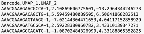
This CSV file has each sample's barcode information, followed by the new UMAP coordinates. The barcodes with a "-1" suffix came from pbmcv1p1, and the barcodes with "-2" suffixes came from pbmcv2. When the data from the two samples were combined, these suffices were added by the cellranger-atac aggr pipeline to distinguish which sample the barcodes belong to.
Import the corrected UMAP projections into the cellranger-atac aggr pipeline output .cloupe into Loupe Browser. Steps of running the pipeline are described at cellranger-atac aggr pipeline. Select the three dots to the right of the pull-down menu, select the "Import Projections" button, and select the CSV file.
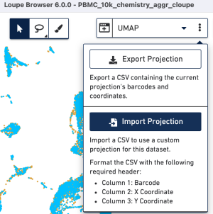
This will give you an updated UMAP visualization.
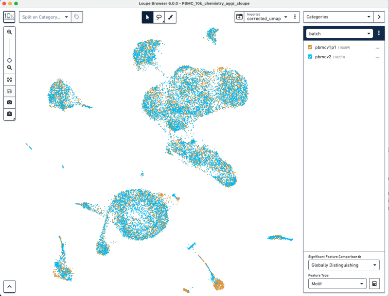
Now, we have used Harmony batch effect correction algorithm to better align the barcodes from pbmcv1p1 and pbmcv2. This batch effect correction removed some of the bias due to technical variation.
Other options for how to handle peaks from different samples:
Since the peak calling was performed on each dataset independently, the peaks are unlikely to be exactly the same. This tutorial used the default peaks from two datasets. If you are interested in using a common set of peaks across all the datasets, you can use the following two methods:
- Obtain a unified set of peaks from samples using
reduce,disjoin, orintersectfunctions from GenomicRanges package. Please refer to Signac Merging object Tutorial. - Redo peak calling using combined data. The cellranger-atac aggr pipeline redo peak calling using data from all input samples. The new output peaks from
aggrpipeline could also be used for downstream batch correction.
aggr_peaks <- read.table(file = "aggr_peaks.bed", col.names = c("chr", "start", "end")) aggr_peaks <- makeGRangesFromDataFrame(aggr_peaks)
After identifying a common set of peaks, you will filter the R object with the common set of peaks based on the Signac Merging object Tutorial, then continue with Step 4 for batch correction.
Other batch correction algorithms
In addition to cellranger-atac aggr and Harmony, there are other Single Cell ATAC data batch correction methods. For example:
- Signac, which uses label transfer between datasets. See more detail in the integration vignettes.
- Liger, which uses quantile normalization. More detail in this tutorial.