Note: 10x Genomics does not provide support for community-developed tools and makes no guarantees regarding their function or performance. Please contact tool developers with any questions. If you have feedback about Analysis Guides, please email analysis-guides@10xgenomics.com.
Xenium is a new in situ platform from 10x Genomics that quantifies spatial gene expression at subcellular resolution. In addition to automated biochemistry and image acquisition, the platform also performs onboard data analysis so raw images are distilled into data points for cells and transcripts.
As part of the onboard data analysis, Xenium automatically performs nucleus segmentation using a custom neural network. The analysis pipeline takes DAPI signals from the 3D image stack into account but ultimately produces a flattened 2D nucleus segmentation mask. It then expands the nuclear boundary by 15 microns in all directions to approximate the cell boundary, and assigns transcripts to a cell if it falls within the cell boundary.
Xenium’s approach approximates cell boundaries using nuclei stains. Customers who have some familiarity with Linux may wish to perform their own cell segmentation using a third-party tool if they are not satisfied with Xenium’s default cell segmentation and transcript mapping. This analysis guide uses Baysor 0.5.2 to perform cell segmentation on Xenium data based on transcriptional composition, and then uses a Python script to create a cell-feature matrix that can be used for downstream data analysis.
This analysis guide requires the following file from the Xenium output folder:
- transcripts.csv.gz
Once the requisite libraries are installed, the first section will provide a Python script to preprocess Xenium’s transcript CSV output and then use Baysor to perform cell segmentation.
The second section will show how to remap transcripts to cells using custom code. The final result is a cell-feature matrix in MTX format that is compatible with popular third-party tools such as Seurat and Scanpy.
Miniconda
We recommend using Miniconda to install Python and manage third-party libraries. Miniconda can be installed by following the directions at: https://docs.conda.io/projects/conda/en/latest/user-guide/install/index.html.
Python libraries
pandaslibrary has data structures that make it easy to work with mixed type tabular data.scipylibrary has support for sparse matrices and it will be used to produce a cell-feature matrix in MTX format.
These libraries can be installed by running the following shell commands:
# Update conda
conda update conda
# Create the xenium conda environment
conda create --name xenium python=3.9.12
# Activate the xenium conda environment
conda activate xenium
# Install libraries
conda install pandas
conda install scipy
# Go back to base environment
conda deactivate
After running the commands above, you should now have a xenium conda environment with the following installed:
python3.9.12pandas1.4.4scipy1.9.1
Baysor 0.5.2
Baysor installation is documented at https://github.com/kharchenkolab/Baysor#installation. However, we encountered multiple problems with those instructions. As a result, we recommend using the alternative instructions below to compile Baysor on your machine. These steps have been verified on a Linux server running Amazon Linux 2, in addition to macOS laptops running Big Sur 11.7.
- Download and install Julia v1.8.3 from https://julialang.org/downloads/. For Linux, we downloaded the glibc link. For macOS, we downloaded the .tar.gz link.
- Expand the tarball.
tar xvfz julia-1.8.3*.tar.gz
- The
juliacommand can be found within the julia-1.8.3/bin/ subfolder. Add that directory to your $PATH environment variable by following these instructions for Linux and macOS. - Run the following shell commands:
# Download GitHub zip file.
curl -L -O https://github.com/kharchenkolab/Baysor/archive/refs/heads/master.zip
# Unzip master.zip, change directory
unzip master.zip
cd Baysor-master
- Run the
juliacommand. On a Mac, you may have to circumvent Gatekeeper (https://support.apple.com/en-us/HT202491) to run the command.
julia
- Within the Julia interactive interpreter, run the following commands:
using Pkg
Pkg.add(Pkg.PackageSpec(;name="PackageCompiler"))
Pkg.activate(".")
Pkg.instantiate()
# Exit Julia
exit()
- Run the following on the shell to compile Baysor. This step can take more than 45 minutes.
julia ./bin/build.jl
- The
Baysorbinary can be found within the Baysor-master/Baysor/bin/ subfolder. Add that directory to your $PATH environment variable. - Check that
Baysoris properly compiled by runningBaysor -h. You should see the following help text:
Usage: baysor <command> [options]
Commands:
run run segmentation of the dataset
preview generate preview diagnostics of the dataset
Alternatively, use Docker to run Baysor. We tested multiple tagged versions from https://hub.docker.com/r/vpetukhov/baysor/tags, and found that vpetukhov/baysor:v0.5.0 is the only container that works reliably. In particular, neither vpetukhov/baysor:latest nor vpetukhov/baysor:master worked.
Preprocessing Xenium’s transcripts.csv.gz
For Baysor, the most relevant Xenium output file is transcripts.csv.gz. The file format is documented online here, and one such file can be downloaded from 10x public datasets. Here are a few quick notes about some of its columns:
-
cell_id: If a transcript is NOT associated with a cell, it will get -1. If it is associated with a cell, this column will have a positive integer cell ID.
-
x_location, y_location, z_location: These three columns store the (x, y, z) coordinates of the transcript in microns. The origin is found in the upper-left corner of the bottom z-slice, as the following image illustrates.
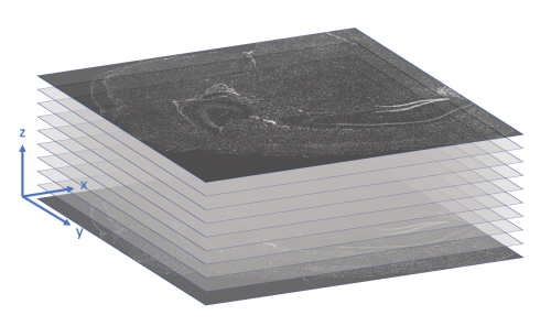
-
feature_name: The gene associated with the transcript.
-
qv: Phred-scaled quality score of all decoded transcripts. It is up to the customer to determine a suitable Q-Score threshold when analyzing Xenium data. At 10x Genomics, we typically filter out transcripts with Q-Score < 20.
Before proceeding further, it is recommended to run the following Python script to preprocess Xenium’s transcript CSV file for Baysor. The script will perform the following:
- Filter out negative control transcripts.
- Filter out transcripts whose Q-Score falls below a specified threshold (default: 20).
- Since Baysor errors out if the cell_id column contains negative integers, it is necessary to modify the cell_id value from -1 to 0 for transcripts that are not associated with cells.
As an added bonus, the script can also be used to subset the dataset (e.g. only keep transcripts whose x_location is < 1000 microns) and facilitate faster iterations of parameter-tuning. To run the script, do the following:
-
Copy and paste the code to a new text file.
#!/usr/bin/env python3 import argparse import sys import pandas as pd def main(): # Parse input arguments. args = parse_args() data_frame = pd.read_csv(args.transcript) # Filter transcripts. Ignore negative controls filtered_frame = data_frame[(data_frame["qv"] >= args.min_qv) & (data_frame["x_location"] >= args.min_x) & (data_frame["x_location"] <= args.max_x) & (data_frame["y_location"] >= args.min_y) & (data_frame["y_location"] <= args.max_y) & (~data_frame["feature_name"].str.startswith("NegControlProbe_")) & (~data_frame["feature_name"].str.startswith("antisense_")) & (~data_frame["feature_name"].str.startswith("NegControlCodeword_")) & (~data_frame["feature_name"].str.startswith("BLANK_"))] # Change cell_id of cell-free transcripts from -1 to 0 neg_cell_row = filtered_frame["cell_id"] == -1 filtered_frame.loc[neg_cell_row,"cell_id"] = 0 # Output filtered transcripts to CSV filtered_frame.to_csv('_'.join(["X"+str(args.min_x)+"-"+str(args.max_x), "Y"+str(args.min_y)+"-"+str(args.max_y), "filtered_transcripts.csv"]), index=False, encoding = 'utf-8') #-------------------------- # Helper functions def parse_args(): """Parses command-line options for main().""" summary = 'Filter transcripts from transcripts.csv based on Q-Score threshold \ and upper bounds on x and y coordinates. Remove negative controls.' parser = argparse.ArgumentParser(description=summary) requiredNamed = parser.add_argument_group('required named arguments') requiredNamed.add_argument('-transcript', required = True, help="The path to the transcripts.csv file produced " + "by Xenium.") parser.add_argument('-min_qv', default='20.0', type=float, help="The minimum Q-Score to pass filtering. (default: 20.0)") parser.add_argument('-min_x', default='0.0', type=float, help="Only keep transcripts whose x-coordinate is greater than specified limit. " + "If no limit is specified, the default minimum value will be 0.0") parser.add_argument('-max_x', default='24000.0', type=float, help="Only keep transcripts whose x-coordinate is less than specified limit. " + "If no limit is specified, the default value will retain all " + "transcripts since Xenium slide is <24000 microns in x and y. " + "(default: 24000.0)") parser.add_argument('-min_y', default='0.0', type=float, help="Only keep transcripts whose y-coordinate is greater than specified limit. " + "If no limit is specified, the default minimum value will be 0.0") parser.add_argument('-max_y', default='24000.0', type=float, help="Only keep transcripts whose y-coordinate is less than specified limit. " + "If no limit is specified, the default value will retain all " + "transcripts since Xenium slide is <24000 microns in x and y. " + "(default: 24000.0)") try: opts = parser.parse_args() except: sys.exit(0) return opts if __name__ == "__main__": main() -
Save the file with a *.py extension (e.g. filter_transcripts.py).
-
Give the script execute permission.
# Give files with .py extension execute permission chmod 755 *.py -
Decompress transcripts.csv.gz and activate the xenium conda environment. Take a look at the script’s help text.
# Decompress transcripts.csv.gz from Xenium output bundle gunzip transcripts.csv.gz # Activate the xenium conda environment conda activate xenium # Get script help text ./filter_transcripts.py -h -
Run the filter script. It will generate a new CSV file with a *_filtered_transcripts.csv filename suffix.
./filter_transcripts.py -transcript transcripts.csv
(optional) Baysor preview command
The Baysor preview command enables a quick overview analysis of your dataset. By default, it creates a preview.html file (modifiable with -o parameter) with plots for transcript, noise, and gene structure. In this section, we run preview to further stress test the binary that was compiled earlier, as well as to gauge how runtime and memory usage scale with dataset size.
Command-line options for Baysor preview are displayed by running Baysor preview -h. In particular, we want to highlight these parameters:
-x,-y,-z: These parameters specify the columns for x, y, z coordinates, respectively. For Xenium data, these columns are named x_location, y_location, and z_location.-g: This parameter specifies the column containing gene names. For Xenium data, it is named feature_name.
A typical call of Baysor preview looks like the following. Please remember to replace TRANSCRIPT_CSV with the path to your transcript CSV file.
# Replace TRANSCRIPT_CSV with actual path to file
Baysor preview -x x_location -y y_location -z z_location -g feature_name TRANSCRIPT_CSV
On an Amazon m5a.24xlarge instance, we observed the following runtime and peak memory usage while varying the number of transcripts:
| Number of Transcripts | 1,232,092 | 2,164,019 | 3,413,020 | 4,661,653 |
|---|---|---|---|---|
| Runtime | 5 min. 37 sec. | 8 min. 3 sec. | 11 min. 17 sec. | 15 min. 17 sec. |
| Peak Memory Usage | 14.6 GB | 22.6 GB | 36.0 GB | 44.1 GB |
As the following plots show, the runtime and peak memory usage of Baysor preview increase linearly with the number of transcripts. Xenium datasets can be large with over 40 million transcripts, so please keep your server’s available memory in mind when processing large datasets.
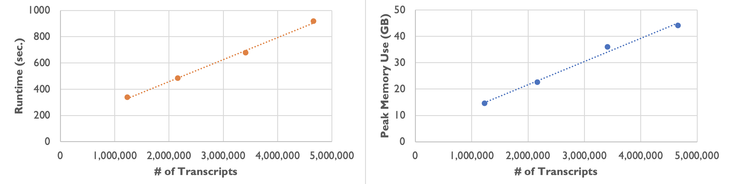
On most Linux servers, the OOM (Out-Of-Memory) Killer would immediately kill the Baysor job if memory usage exceeds what is available on the server. On a Mac computer with root access, jobs are able to run to completion but runtime increases even more steeply once the computer is forced to use slower virtual memory.
Baysor run command
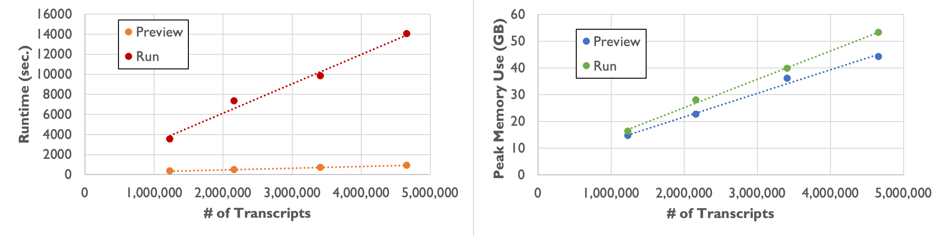
The Baysor run command performs cell segmentation based on transcriptional composition. Because the algorithm runs hundreds of iterations until the results converge, runtime is significantly longer compared to the preview command.
As shown in the following table and plot, runtime and peak memory usage of Baysor run increase linearly with the number of transcripts. Compared to the preview command, runtime increases more than tenfold, while peak memory usage remains similar.
| Number of Transcripts | 1,232,092 | 2,164,019 | 3,413,020 | 4,661,653 |
|---|---|---|---|---|
| Runtime | 58 min. 49 sec. | 2 hr. 1 min. 53 sec. | 2 hr. 43 min. 38 sec. | 3 hr. 53 min. 49 sec. |
| Peak Memory Usage | 16.3 GB | 27.9 GB | 39.8 GB | 53.2 GB |
Command-line options for Baysor run are displayed by running Baysor run -h. In particular, we want to highlight these parameters:
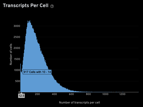
-x,-y,-z: These parameters specify the columns for x, y, z coordinates, respectively. For Xenium data, these columns are named x_location, y_location, and z_location.-g: This parameter specifies the column containing gene names. For Xenium data, it is named feature_name.-m: This parameter specifies the minimum number of transcripts that is expected from a real cell. This is an important value since it is used to infer several other parameters. The optimal setting will be sample-dependent, but the Xenium analysis web summary contains a Transcripts Per Cell plot under the Cell Segmentation tab that can help in determining a suitable value. The plot usually has a narrow peak with low transcript count from “noisy” cells, and a main peak from genuine cells. Given a plot like the one shown below, you can hover the cursor over it to display extra info. In this case,-m 15seems like an appropriate setting.
-s: This parameter specifies the approximate cell radius for the algorithm. In our experience, this parameter has an outsized effect on segmentation results. It is better NOT to set this parameter if the sample contains cells of different sizes. In the table below, you can see how much it affects the final result.
| -s Setting | Xenium | 5 | 10 | 15 |
|---|---|---|---|---|
| Segmentation Result |  |  | 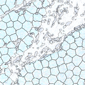 |  |
--prior-segmentation-confidence: Baysor can use prior segmentation results, such as the one produced by Xenium. This parameter ranges from 0 to 1, where 1 means that Baysor cannot contradict the prior segmentation. For Xenium data, cell segmentation results are stored in the cell_id column. The optimal setting will be sample-dependent, so we recommend starting with 0.5, and fine-tune as needed.
Putting everything together, a typical Baysor run would look like the following. Please remember to replace capitalized inputs (MIN_TRANSCRIPT, PRIOR_CONF, TRANSCRIPT_CSV) with suitable arguments.
# Replace MIN_TRANSCRIPT, PRIOR_CONF, and TRANSCRIPT_CSV before running
Baysor run -x x_location -y y_location -z z_location -g feature_name -m MIN_TRANSCRIPT -p --prior-segmentation-confidence PRIOR_CONF TRANSCRIPT_CSV :cell_id
Once Baysor performs cell segmentation, it is necessary to remap all the transcripts to cells in order to conform with the redefined cell boundaries.
The Python script below will perform these tasks:
- Process all transcripts from *segmentation.csv produced by Baysor, and filter out entries that fall below a user-specified assignment confidence threshold.
- Generate a cell-feature matrix and output that matrix in a MTX format that is compatible with Seurat and Scanpy.
Running the script with -h displays the help text that lists the required and optional parameters. This script should be run using the xenium conda environment.
#!/usr/bin/env python3
import argparse
import csv
import os
import sys
import numpy as np
import pandas as pd
import scipy.sparse as sparse
import scipy.io as sio
import subprocess
def main():
# Parse input arguments.
args = parse_args()
# Check for existence of input file.
if (not os.path.exists(args.baysor)):
print("The specified Baysor output (%s) does not exist!" % args.baysor)
sys.exit(0)
# Check if output folder already exist.
if (os.path.exists(args.out)):
print("The specified output folder (%s) already exists!" % args.out)
sys.exit(0)
# Read 5 columns from transcripts Parquet file
transcripts_df = pd.read_csv(args.baysor,
usecols=["gene",
"cell",
"assignment_confidence"])
# Find distinct set of features.
features = np.unique(transcripts_df["gene"])
# Create lookup dictionary
feature_to_index = dict()
for index, val in enumerate(features):
feature_to_index[str(val)] = index
# Find distinct set of cells. Discard the first entry which is 0 (non-cell)
cells = np.unique(transcripts_df["cell"])[1:]
# Create a cells x features data frame, initialized with 0
matrix = pd.DataFrame(0, index=range(len(features)), columns=cells, dtype=np.int32)
# Iterate through all transcripts
for index, row in transcripts_df.iterrows():
if index % args.rep_int == 0:
print(index, "transcripts processed.")
feature = str(row['gene'])
cell = row['cell']
conf = row['assignment_confidence']
# Ignore transcript below user-specified cutoff
if conf < args.conf_cutoff:
continue
# If cell is not 0 at this point, it means the transcript is associated with a cell
if cell != 0:
# Increment count in feature-cell matrix
matrix.at[feature_to_index[feature], cell] += 1
# Call a helper function to create Seurat and Scanpy compatible MTX output
write_sparse_mtx(args, matrix, cells, features)
#--------------------------
# Helper functions
def parse_args():
"""Parses command-line options for main()."""
summary = 'Map Xenium transcripts to Baysor segmentation result. \
Generate Seurat/Scanpy-compatible feature-cell matrix.'
parser = argparse.ArgumentParser(description=summary)
requiredNamed = parser.add_argument_group('required named arguments')
requiredNamed.add_argument('-baysor',
required = True,
help="The path to the *segmentation.csv file produced " +
"by Baysor.")
requiredNamed.add_argument('-out',
required = True,
help="The name of output folder in which feature-cell " +
"matrix is written.")
parser.add_argument('-conf_cutoff',
default='0.9',
type=float,
help="Ignore transcripts with assignment confidence " +
" below this threshold. (default: 20.0)")
parser.add_argument('-rep_int',
default='100000',
type=int,
help="Reporting interval. Will print message to stdout " +
"whenever the specified # of transcripts is processed. " +
"(default: 100000)")
try:
opts = parser.parse_args()
except:
sys.exit(0)
return opts
def write_sparse_mtx(args, matrix, cells, features):
"""Write feature-cell matrix in Seurat/Scanpy-compatible MTX format"""
# Create the matrix folder.
os.mkdir(args.out)
# Convert matrix to scipy's COO sparse matrix.
sparse_mat = sparse.coo_matrix(matrix.values)
# Write matrix in MTX format.
sio.mmwrite(args.out + "/matrix.mtx", sparse_mat)
# Write cells as barcodes.tsv. File name is chosen to ensure
# compatibility with Seurat/Scanpy.
with open(args.out + "/barcodes.tsv", 'w', newline='') as tsvfile:
writer = csv.writer(tsvfile, delimiter='\t', lineterminator='\n')
for cell in cells:
writer.writerow(["cell_" + str(cell)])
# Write features as features.tsv. Write 3 columns to ensure
# compatibility with Seurat/Scanpy.
with open(args.out + "/features.tsv", 'w', newline='') as tsvfile:
writer = csv.writer(tsvfile, delimiter='\t', lineterminator='\n')
for f in features:
feature = str(f)
if feature.startswith("NegControlProbe_") or feature.startswith("antisense_"):
writer.writerow([feature, feature, "Negative Control Probe"])
elif feature.startswith("NegControlCodeword_"):
writer.writerow([feature, feature, "Negative Control Codeword"])
elif feature.startswith("BLANK_"):
writer.writerow([feature, feature, "Blank Codeword"])
else:
writer.writerow([feature, feature, "Gene Expression"])
# Seurat expects all 3 files to be gzipped
subprocess.run("gzip -f " + args.out + "/*", shell=True)
if __name__ == "__main__":
main()
If the script above is saved to a file called map_transcripts.py, then a sample invocation might look like the following:
# Activate the xenium conda environment
conda activate xenium
# Map transcripts to cells
./map_transcripts.py -baysor baysor_segmentation.csv -out baysor_mtx
After running the Python transcript mapping script, the resulting cell-feature matrix can be read by popular third-party tools such as Seurat and Scanpy.
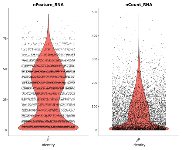
To demonstrate compatibility, we were able to follow this Seurat vignette and use the Read10X() function to load the matrix. We produced the following plots after using Baysor to redo cell segmentation for the upper-left 1000 by 1000 micron region of a breast cancer dataset, and it should be straightforward to cluster the cells, generate a UMAP projection, and find differentially expressed features.
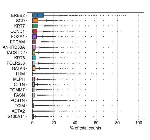
Likewise, we were able to follow this Scanpy tutorial and use the read_10x_mtx() function to load the matrix. The following plot shows the 20 genes that have the highest fraction of counts in each cell in the upper-left 1000 by 1000 micron region, and it should be straightforward to proceed further with the tutorial and run the standard suite of single cell data analysis with this cell-feature matrix.