This page describes raw output (decoded transcript counts and morphology images) and other standard output files derived from them, which are included in the Xenium output directory for each selected region (also see Archiving Xenium data). These data reduce low-level internal image sensor data, preserving details needed to assess decoded transcript quality (learn more at Overview of Xenium Algorithms).
All run data will be stored in the output/ directory on the Xenium Analysis Computer and will be accessible on the Desktop. Refer to the Xenium Instrument User Guide (CG000584) for instructions to export run data from the instrument.
Within the output/ directory, the data from individual runs are stored as subfolders and include the user-defined run name in the folder name. Within the top-level run folder, there are subfolders for each of the user-defined regions on the Xenium slides. The overall organization of subfolders is shown below:
output
└── <yyyymmdd>__<hhmmss>__<runName>
└── output-<instrumentSN>__<slideID>__<regionName>__<yyyymmdd>__<hhmmss>
The runName and regionName strings are user-defined; the other components of the directory names are auto-generated. <yyyymmdd> is the start date and <hhmmss> is the start time (in UTC). The separators between the strings in the directory name are two underscores. Spaces in runName and regionName will be replaced by an underscore (_) in the output directory name.
The remaining sections describe the Xenium output bundle files for each analysis run.
The experiment.xenium is an experiment manifest file in JSON format that includes experiment metadata and relative file paths to other data files in the output folder needed by Xenium Explorer to visualize results.
Click the link below for metadata descriptions.
XOA v4.0 generates protein data-specific files, along with modifications to the gene expression outputs, for data generated with the Xenium In Situ Gene and Protein Expression with Cell Segmentation Staining assay (CG000819).
Click the link below for protein data-specific output descriptions.
The Xenium onboard analysis pipeline outputs an interactive HTML file named analysis_summary.html. Open it on-instrument, in a web browser, or in Xenium Explorer. It contains summary metrics and automated secondary analysis results. Any alerts issued by the pipeline are displayed at the top of the page.
There are five clickable tabs:
- The Summary tab contains summary metrics, images, and experiment information for a quick overview of the data.
- The Decoding tab contains transcript decoding metrics and plots.
- The Cell Segmentation tab shows metrics for cell segmentation and partitioning transcripts into single cells.
- The Analysis tab captures the results from the pipeline's secondary analysis run on single cell data.
- The Image QC tab contains several image galleries, including downsampled RNA images for each cycle and channel, morphology stain images, and background autofluorescence images.
Click the ? at the top of each dashboard for more information about each metric. For detailed descriptions and guidance on interpretation, click below.
A series of tissue morphology images are output by the pipeline, which are either nuclei-stained (DAPI) or nuclei and multi-tissue stained (DAPI, cell boundary, interior stains) images in OME-TIFF format. These files include a pyramid of resolutions and tiled chunks of image data, which allows for efficient interactive image visualization (JPEG-2000 compression, 16-bit grayscale, full and downsampled resolutions down to 256 x 256 pixels, learn more here).
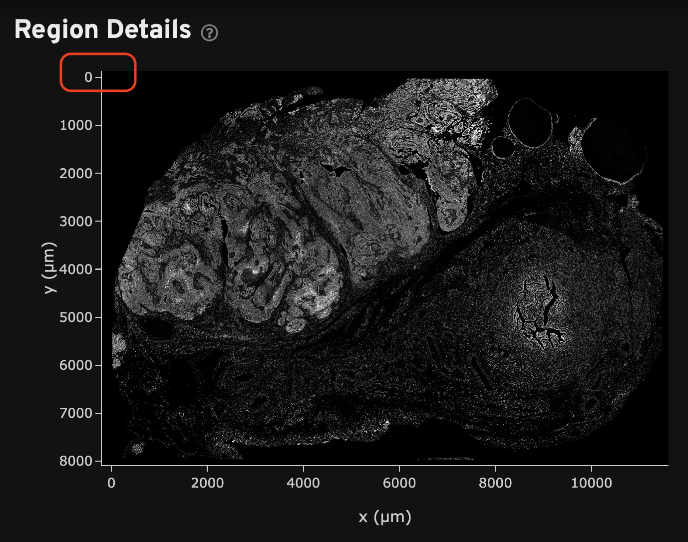
All Xenium morphology images are oriented with the origin (0,0) in the top left corner (image coordinate system). For reference, the image axes are labeled in the Summary and Image QC tabs of the analysis summary file. The transcript X, Y, and Z locations use the same image coordinate system orientation.
- The
morphology.ome.tifis a 3D Z-stack of the DAPI image that can be useful to resegment cells, assess segmentation quality, and view data. DAPI image processing is described here. - The
morphology_focus/directory contains the 2D autofocus projection images for the nuclei DAPI stain image, as well as additional stain images for Xenium outputs generated with multimodal cell segmentation assay workflows. These files are in multi-file OME-TIFF format. They each contain a pyramid of images including full resolution and downsampled images. Learn about 2D image processing here. The image order is specified in OME-XML metadata.
Here is an example of the cell segmentation marker images:
morphology_focus/
├── ch0000_dapi.ome.tif (DAPI)
├── ch0001_atp1a1_e-cadherin_cd45.ome.tif (ATP1A1/E-Cadherin/CD45)
├── ch0002_18s.ome.tif (18S rRNA)
└── ch0003_alphasma_vimentin.ome.tif (alphaSMA/Vimentin)
For details on 2D morphology images generated for the Xenium In Situ Gene and Protein Expression with Cell Segmentation Staining assay, see this page.
The OME-TIFF morphology image files can be viewed in Xenium Explorer. The image orientation is the same as shown in the analysis summary, with the origin in the top left corner. This is relevant for image alignment and explained further in the alignment tutorial.
Multi-file OME-TIFF images can also be viewed in community-developed visualization software such as QuPath, Napari, or Fiji/ImageJ. To view all focus images in these programs, simply open one of the files (i.e., open program, drag and drop ch0000_dapi.ome.tif file). Since each focus image file's metadata specifies that all the focus files are stored in the morphology_focus/ directory, they do not need to be imported separately.
morphology_focus directory contains ALL the images (e.g., QuPath), while others will open with fewer than the total (e.g., Napari, where missing images display as blanks).Programmatic examples for viewing these files is provided below.
If needed, multi-file images can also be converted to a single stack OME-TIFF format, for example by following these QuPath and Tifffile file conversion instructions.
The cell summary file (cells.csv.gz) in gzipped CSV format contains data to help QC the transcript counts for each identified cell. The file contains one row for each cell, with the following columns:
| Column Name | Description |
|---|---|
cell_id | Unique ID of the cell, consisting of a cell prefix and dataset suffix |
x_centroid | X location of the cell centroid in µm |
y_centroid | Y location of the cell centroid in µm |
transcript_counts | Molecule count of gene features with Q-Score ≥ 20 |
control_probe_counts | Molecule count of negative control probes |
genomic_control_counts | Count of genomic control codewords (for Xenium Prime data) |
control_codeword_counts | Count of negative control codewords |
unassigned_codeword_counts | Count of unassigned codewords |
deprecated_codeword_counts | Count of deprecated codewords |
total_counts | Sum total of transcript_counts, control_probe_counts, control_codeword_counts, genomic_control_counts (for Xenium Prime data), and unassigned_codeword_counts |
cell_area | The two-dimensional area covered by the cell in µm2 |
nucleus_area | The two-dimensional area covered by the nucleus in µm2 |
nucleus_count | Count of detected nuclei |
segmentation_method | Cell segmentation method |
The cell summary is also provided in Parquet format (cells.parquet) to enable faster loading and reading of data (code examples here).
Nucleus boundaries are determined by a nucleus segmentation algorithm that runs on the nuclei-stained (DAPI) morphology image. Cell boundaries are either determined by 1) expanding the nucleus boundaries 5 µm or until the expanded boundary hits another cell, or 2) using boundary and interior cell stains.
The cells.zarr.zip file in zipped Zarr format contains segmentation masks and boundaries for nuclei and cells. These segmentation masks are used for assigning transcripts to cells. The boundary polygons are approximations of the segmentation masks, and are provided for efficient visualization of cell segmentation in Xenium Explorer and other analysis software. See Overview of Xenium Zarr Output Files for file specifications.
The nucleus_boundaries.csv.gz and cell_boundaries.csv.gz are the CSV representation of the nucleus and cell boundaries, respectively. Each row represents a vertex in the boundary polygon of one cell. The boundary points for each cell appear in clockwise order, and the first and the last points are duplicates to indicate a closed polygon. Both files contain the following columns:
| Column Name | Description |
|---|---|
cell_id | Unique ID of the cell, consisting of a cell prefix and dataset suffix |
vertex_x | X-coordinate of the boundary point in µm |
vertex_y | Y-coordinate of the boundary point in µm |
label_id | A nonzero number corresponding to the segmentation mask pixel value |
The same nucleus and cell boundary information is also provided in Parquet format (nucleus_boundaries.parquet and cell_boundaries.parquet) to enable faster loading and reading of data (code examples here).
The transcripts file (transcripts.parquet) contains data to evaluate transcript quality and localization based on the image coordinate system of the morphology images. It is provided in Parquet format to enable faster loading and reading of data (code examples here). The file contains one row for each decoded transcript, with the following columns:
| Column Name | Description |
|---|---|
transcript_id | Unique ID of the transcript |
cell_id | Unique ID of the cell, consisting of a cell prefix and dataset suffix |
overlaps_nucleus | Binary value to indicate if the transcript falls within the segmented nucleus of the cell (1) or not (0) |
feature_name | Gene or control name |
x_location | X location in µm |
y_location | Y location in µm |
z_location | Z location in µm |
qv | Phred-scaled quality value (Q-Score) estimating the probability of incorrect call |
fov_name | Name of the field of view (FOV) that the transcript falls within |
nucleus_distance | The distance between the transcript and the nearest nucleus boundary in µm based on segmentation mask boundaries. The nearest nucleus may not necessarily belong to the cell that the transcript is assigned to. Transcripts localized within the nucleus have a distance of 0.0 µm. |
codeword_index | An integer index for each codeword used to decode transcripts (same value as codewords in the gene_panel.json file). |
codeword_category | Codeword category |
is_gene | Boolean value to indicate whether transcript feature is "Gene Expression" or not. |
Transcript information is also provided in zipped Zarr format (transcripts.zarr.zip). This file can be read by Xenium Explorer. See Overview of Xenium Zarr Output Files for file specifications.
The Xenium onboard analysis pipeline outputs a cell-feature matrix (cell_feature_matrix) in three file formats: the Market Exchange Format (MEX), the Hierarchical Data Format (HDF5), and the Zarr format. The matrices only include transcripts that pass the default quality value (Q-Score) threshold of Q20 and are assigned to cells.
Each matrix in the cell_feature_matrix/ folder is stored in the MEX format for sparse matrices. It also contains gzipped TSV files with feature and barcode sequences corresponding to row and column indices respectively. The cell_feature_matrix/features.tsv.gz file contains a list of pre-designed panel genes (and any custom add-on genes), negative controls, unassigned codewords, and deprecated codewords (learn more about control and codeword categories on the Algorithms page).
XOA v4.0 includes protein features in the cell-feature matrix outputs for data generated with the Xenium In Situ Gene and Protein Expression with Cell Segmentation Staining assay, see this page for details.
| Column Number | Description |
|---|---|
| 1 | Ensembl ID for panel and add-on genes |
| 2 | Gene name for panel and add-on genes |
| 3 | Feature type (Gene Expression, Negative Control Codeword, Negative Control Probe, Genomic Control, Unassigned Codeword, Deprecated Codeword, Protein Expression). |
The cell-feature matrix is also provided in:
- HDF5 format (
cell_feature_matrix.h5), a binary format that compresses and accesses data more efficiently than text formats such as MEX and is useful when analyzing large datasets. H5 files are supported in both R and Python. - Zipped Zarr format (
cell_feature_matrix.zarr.zip). This file can be read by Xenium Explorer. See Overview of Xenium Zarr Output Files for file specifications.
The Xenium onboard analysis pipeline outputs key metrics in text format as metrics_summary.csv. This file contains metrics that are useful for assessing decoding and cell segmentation quality.
The Xenium onboard analysis pipeline outputs an analysis/ directory with subdirectories containing several CSV files, which store the automated secondary analysis results. A subset of these results is used to render the Analysis tab in the Analysis summary file (UMAP, clustering, and differential expression results). The subdirectories are listed below. The file prefixes indicate the type of data input, either gene_expression_ or protein_expression_. Protein data secondary analysis is described here.
- Clustering (
clustering/) with graph-based and K-means results. Graph-based clustering (undergraphclust) is run once as it does not require a pre-specified number of clusters. K-means (underkmeans) is run for K=2..N where K corresponds to the number clusters, and N=10 by default. Each value of K has its own results directory. - Differential Expression (
diffexp/) with graph-based and K-means results. Under each of the subdirectories are thedifferential_expression.csvfiles, which contain the list of cluster-specific features that are differentially expressed in each cluster relative to all the other clusters. - Principal Component Analysis (
pca/) which contains a total of five files listing the features used in the dimension reduction i.e., to reduce the feature space. These results are used to perform clustering. - UMAP (
umap/) contains the Uniform Manifold Approximation and Projection results.
The secondary analysis results are also saved as a zipped Zarr file (analysis.zarr.zip), which can be read by Xenium Explorer for data visualization of graph-based and K-means cluster results. See Overview of Xenium Zarr Output Files for file specifications.
The gene_panel.json file is a copy of the pre-designed or custom gene panel file used in the experiment on the Xenium Analyzer instrument.
- The JSON files and additional resources for 10x pre-designed panels are provided on the pre-designed Xenium Gene Expression Panel pages: v1, Xenium Prime 5K.
- For custom panels, the JSON file can be downloaded from the Xenium Panel Designer tool after the design is finalized. See Getting started with Xenium Panel Design for guidance.
The JSON schema contains metadata and payload objects (code example here for extracting information from the payload object). The payload object contains the following:
| Object | Description |
|---|---|
chemistry | Version of Xenium In Situ assay chemistry (i.e., "v1" for Xenium v1 RNA-only and RNA + Protein, "v2" for Xenium Prime). |
customer | Customer contact information derived from design or 10x cloud if the Xenium Panel Designer was used. |
designer | When and who created the design. |
panel | Information about the panel design, including name, ID, and total number of targets. |
spec_version | Version of panel JSON file format. |
targets | Information about each target (gene, control) in the panel, including gene identifiers and gene coverage (also referred to as the number of probe sets). The latter may be useful for assessing per-gene sensitivity. |
The following are provided in aux_outputs/ (see release notes for updates):
-
The
morphology_fov_locations.jsonfile contains the field of view (FOV) name, height, width, and XY positions in the space of the region of interest's (ROI) morphology image. This is the same space used to compute transcript and cell locations and the units are in microns. The FOVs have 3,520 rows and 2,960 columns with 128 pixels of overlap on each edge (this may change in future versions of the Xenium platform). The position information is useful for determining where FOV boundaries are to assess transcript deduplication and any FOV edge effects. -
The
overview_scan_fov_locations.jsonfile contains the FOV name, height, width, and approximate XY positions in the space of the overview scan image. This is the space that contains all the ROIs and the units are in pixels. The accuracy of the ROI coordinates have a 5 - 10 µm error. This position information is useful for approximating where multiple ROIs are located on an overview scan image. -
The
per_cycle_channel_images/directory contains downsampled 2D RNA images (maximum intensity projection) from each cycle and channel (not the morphology stain images). These images may be helpful for troubleshooting analysis summary alerts or unexpected metrics and analysis results. -
The
overview_scan.pngis the full-resolution (1672 x 3498 pixels) image of the entire sample on the slide. -
The
morphology_focus_qc_masks/directory contains saturation QC mask images. The mask format is 8-bit multi-file OME TIFF, mirroring themorphology_focus/image format. There is one file permorphology_focusimage, and the file names and order are identical to the files in themorphology_focus/directory. For RNA-only datasets, these files provide a record of the image processing masking step (DAPI-only datasets will only contain zeroes. DAPI & cell segmentation datasets may contain saturated pixels, but this is not expected to be common). For protein datasets, these masks can be useful for data QC (read more in protein data outputs). -
The
background_qc_images/directory contains the autofluorescence images that are subtracted from the raw morphology stain images to produce the autofocused images (morphology_focus/) if Cell Segmentation Staining protocol used. These are downsampled, maximum intensity projection (MIP) images (not deconvolved) in TIFF format.└── background_qc_images ├── background_01_blu.tiff ├── background_01_grn.tiff ├── background_01_nuv.tiff └── background_01_red.tiff
The downsampled images use a scale factor of 3.4 µm per pixel. This corresponds to level 4 or Fiji series 5 in this table.
Additional aux_outputs/ image files generated for the Xenium In Situ Gene and Protein Expression with Cell Segmentation Staining assay are described on this page.