The Visium Spatial Gene Expression solution generates spatial, whole-transcriptome data, but each spot typically covers multiple cells. To analyze data at cell type resolution, emerging spot deconvolution methods use single cell reference data to break down Visium spots into their respective cell types (reviewed in this 10x Analysis Guide). Space Ranger v2.1 and Loupe Browser v6.5 take this a step further and introduce combined support for the reference-free spot deconvolution feature, a convenient alternative for when a single cell reference is not available, or to visualize cell-type data directly without relying on third-party tools. The algorithm is built on latent Dirichlet allocation (LDA).
Space Ranger's spot decovolution predicts latent topics that can be thought of as inferred cell types or mixtures of cell types. The outputs are now provided from every spaceranger count and spaceranger aggr run; no special options or parameters are needed. The outputs in the deconvolution/ folder can be used to annotate topics with biological cell types, as described below.
- Learn how to get started with reference-free spot deconvolution using a public mouse brain dataset
- Understand how to view, annotate, and interpret latent topics in Loupe Browser v6.5
- Understand how to use the
deconvolution/outputs to further interpret your results
This introductory tutorial requires only one software installation (Loupe Browser v6.5 and later) for Windows or Mac. No command line environment is required.
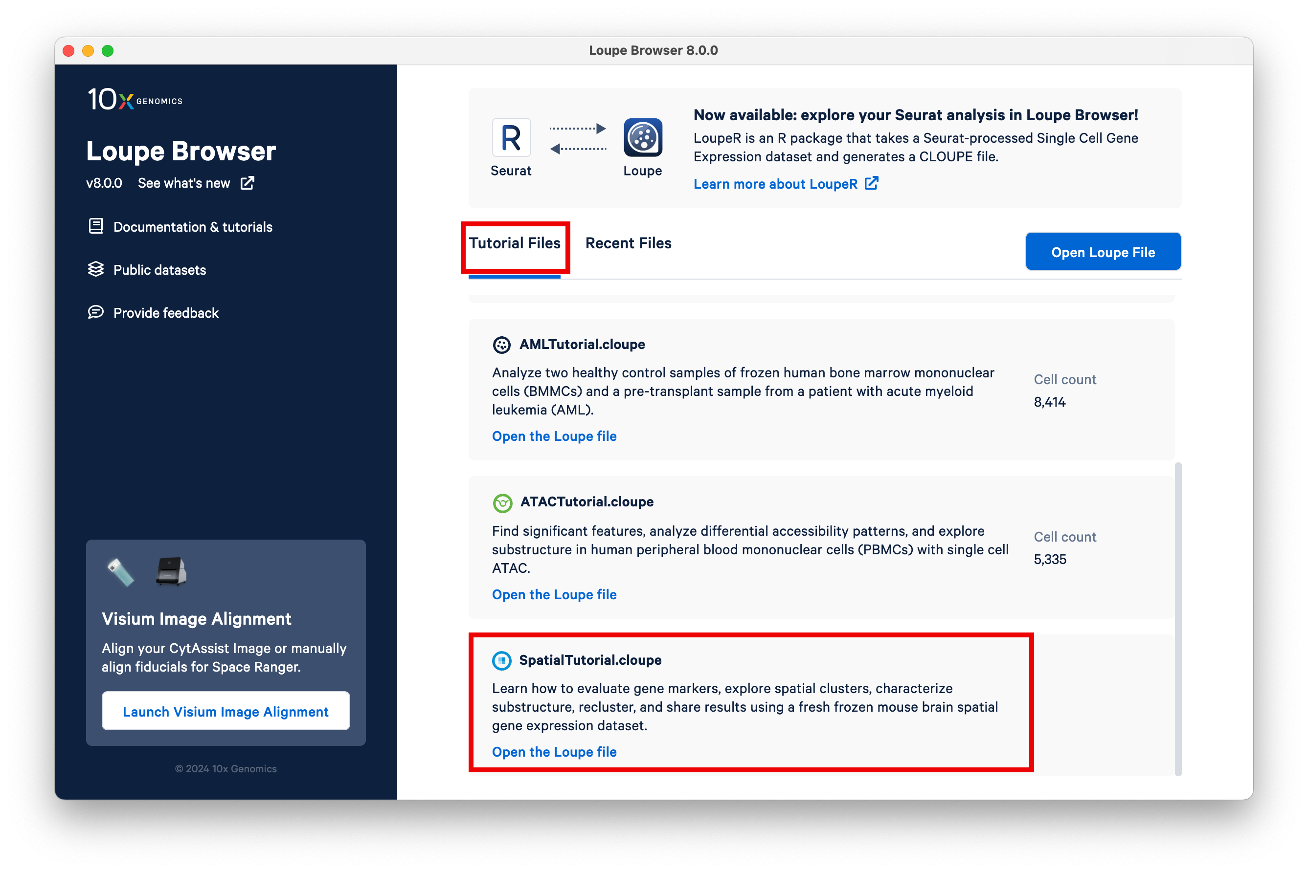
Once you have downloaded and installed Loupe Browser v6.5 on your system, open the bundled Spatial tutorial from the landing screen.
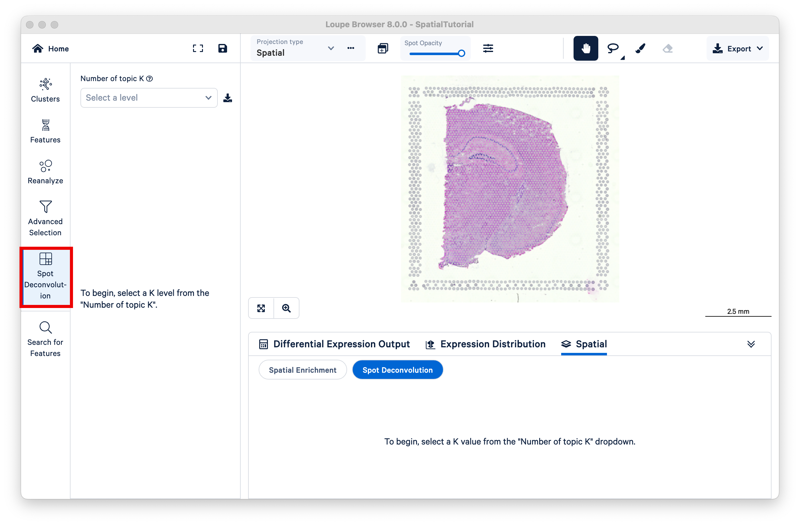
This will open the mouse brain tutorial dataset. By default, the categories loaded are the graph-based clusters. To load the spot deconvolution results, select Spot Deconvolution on the left.
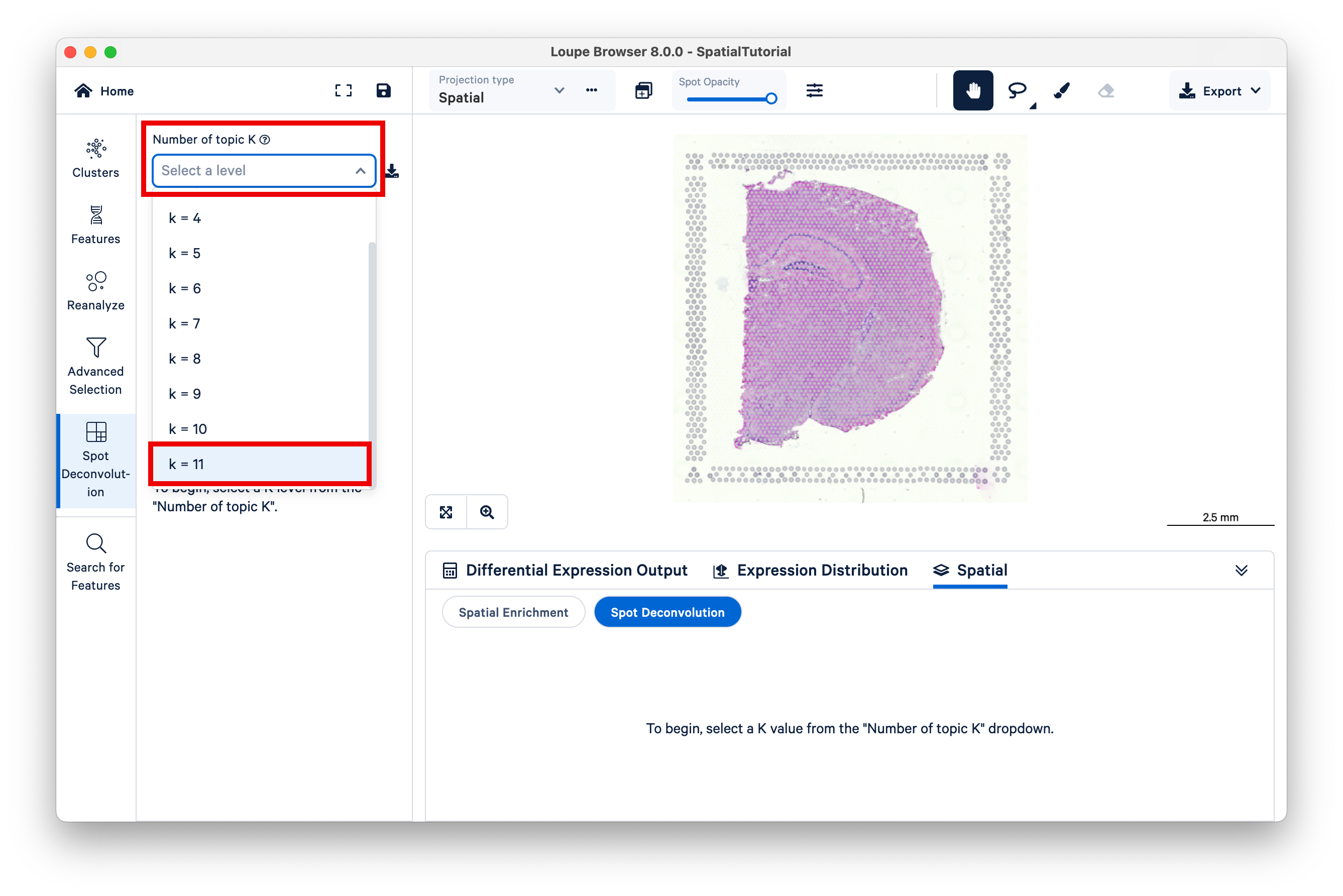
The resulting view is similar to that of graph-based or K-means clustering, but now K represents different topics; deconvolution results are hierarchically clustered by K to reflect different granularity of cell typing. Under the dropdown titled Number of topic K, select k=11.
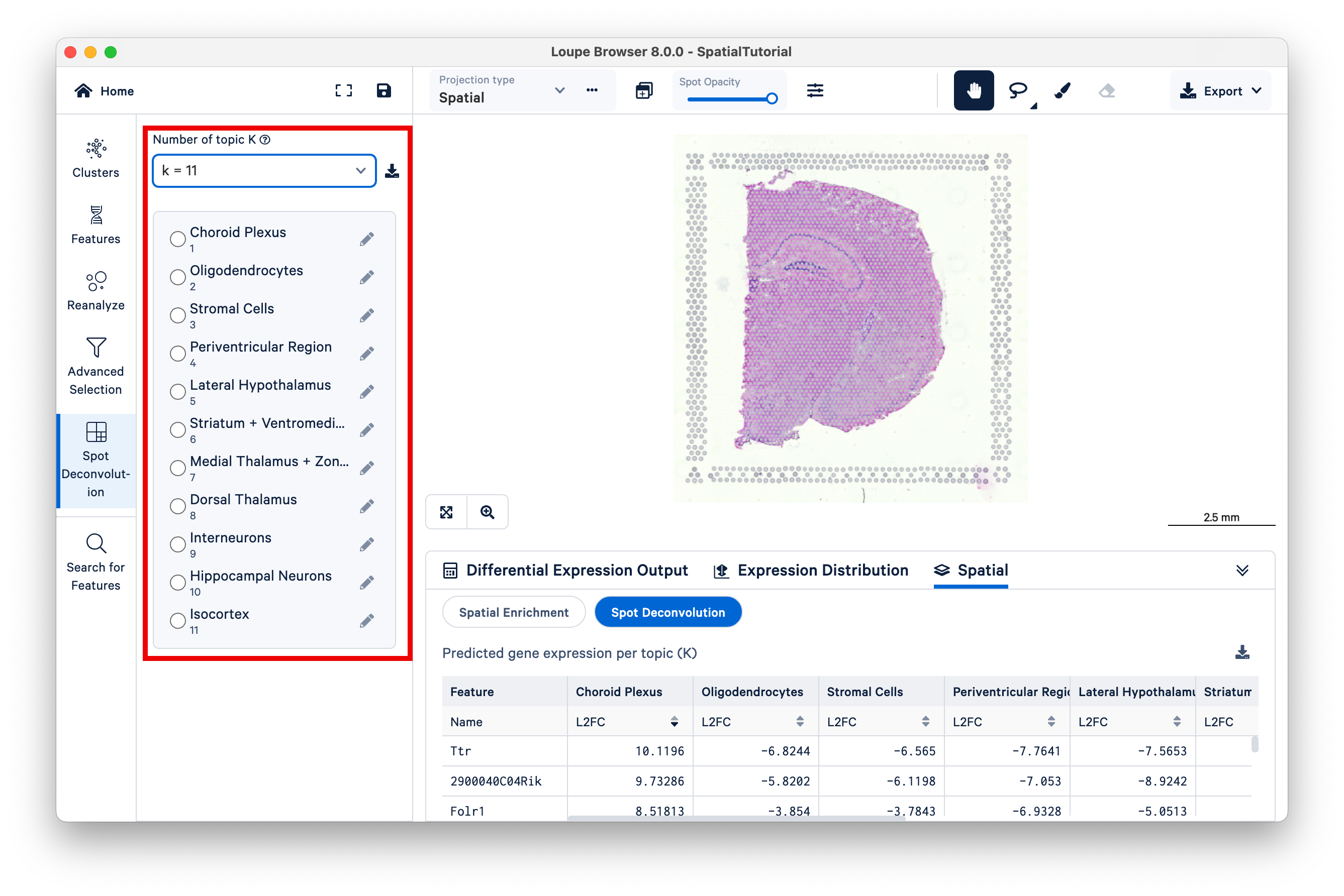
Observe that different topics are annotated as different cell types, or mixtures of cell types, in the mouse brain. (For this dataset, 10x has pre-annotated the topics to cell type; for more information on this topic see the 10x Analysis Guide on web resources for cell type annotation).
Next, select Topic 10 (Hippocampal Neurons). The hippocampus is one of the most prominent features of the mouse brain. You may wish to reduce the saturation of the tissue image to zero to make the colors pop out more.
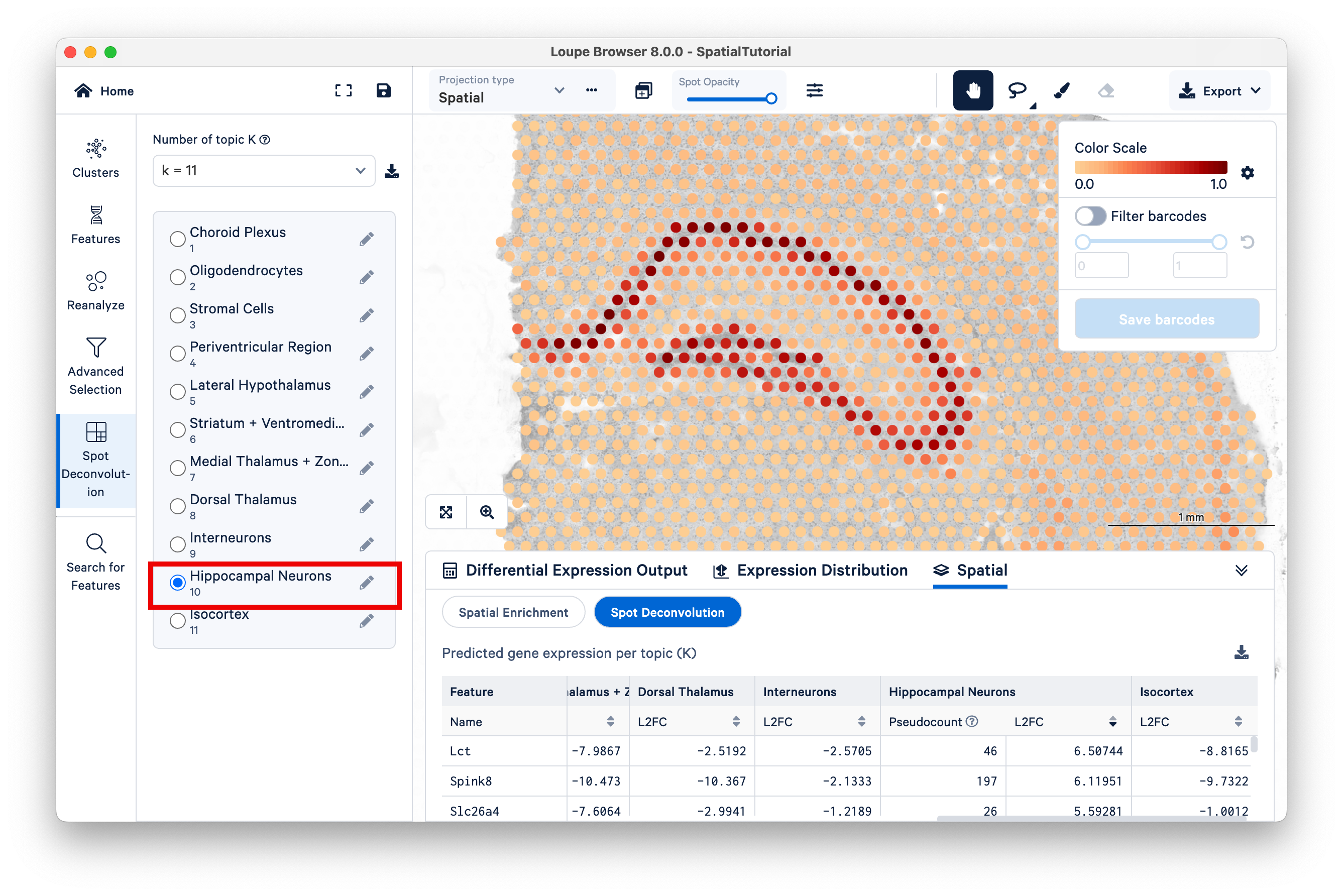
Zoom in to the hippocampus. The color scale on the top right ranges from a value of 0.0 to 1.0, representing the proportion of the spot's expression profile that can be assigned to the selected topic (in this case, topic 10).Notice that the spots that have higher scores for this topic lie along the most visible part of the hippocampus, while spots in adjacent areas have mid-range scores, and spots with very low scores are found across the rest of the tissue.
Another starting point to explore latent topics is to compare the results under different K values. In this tutorial, 10x annotated all the topics under K=11, but under other K values, not all topics are annotated. As K decreases, topics begin to represent more generalized cell types or mixtures of cell types that could reflect tissue-level structures. For example, consider Topic 5, Lateral Hypothalamus under K=11.
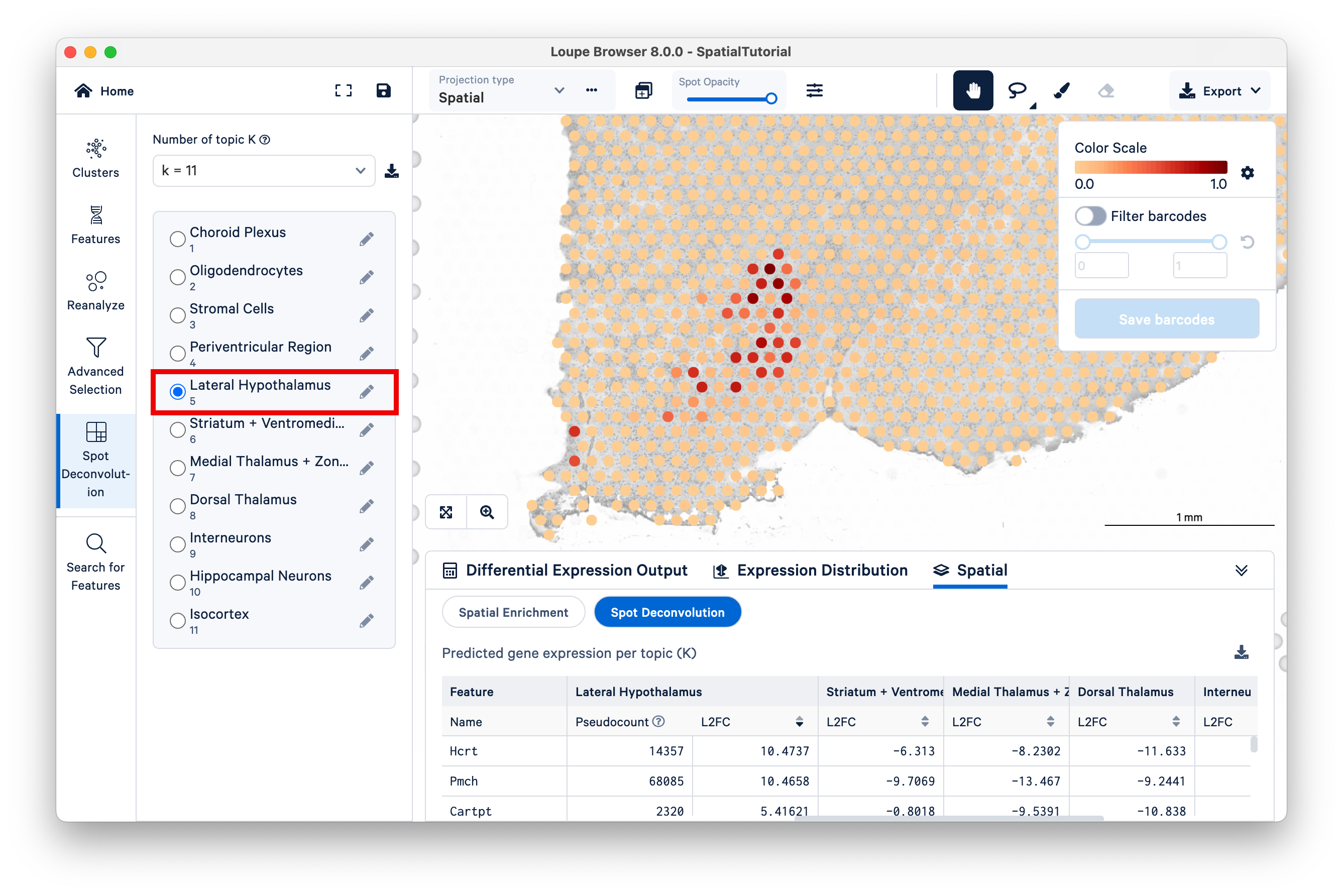
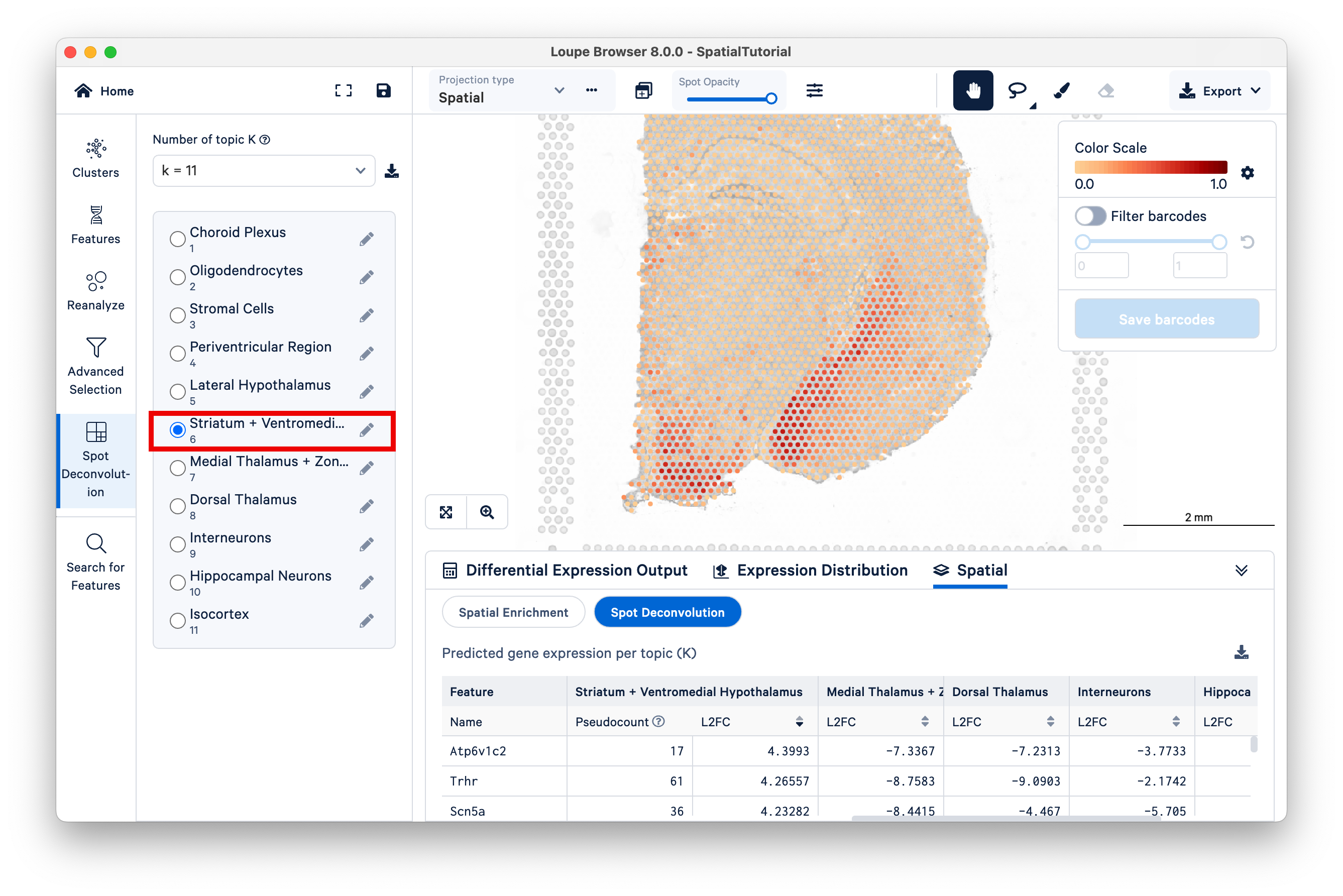
Locate the position of the spots with high scores for this topic on the bottom left region of the tissue. While remaining under K=11, switch to Topic 6, Striatum + Ventromedial Hypothalamus. Zoom out a bit to see which spots are lighting up for this topic.
Now switch to K=9, and select the 5to6 topic. This topic was not annotated, but based on our observations from K=11 and the current view under K=9, observe that this topic represents the lateral hypothalamus, striatum, and ventromedial hypothalamus combined.
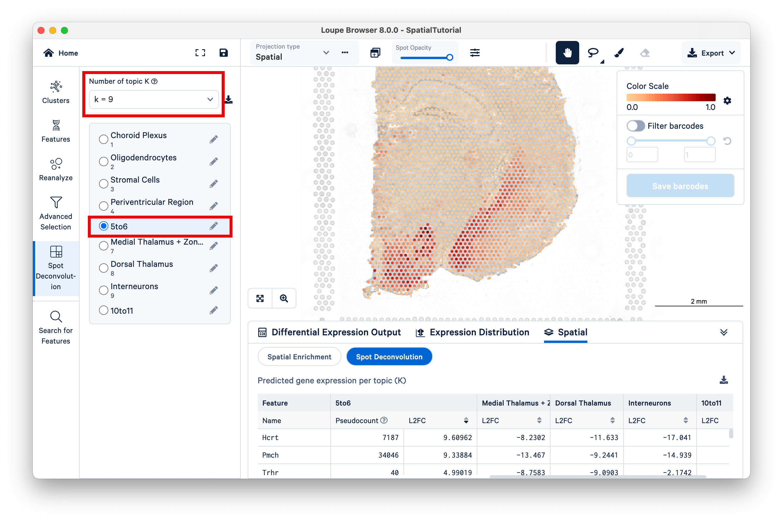
You can annotate this topic manually as "hypothalamus".
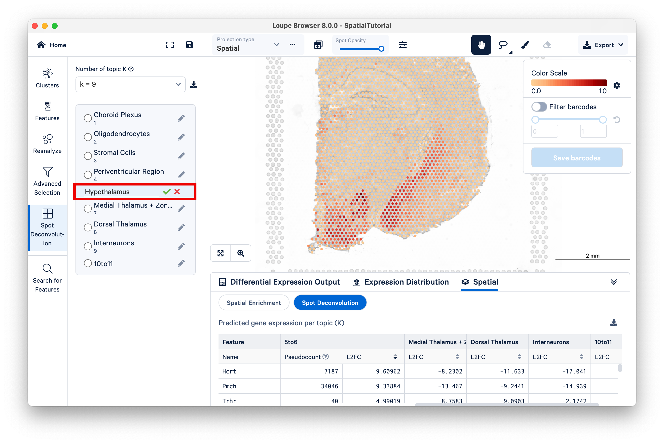
This example illustrates how Space Ranger spot deconvolution results are hierarchically clustered by K to reflect different granularity of cell typing and how users can customize annotations.
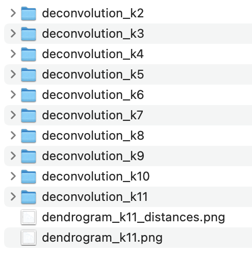
In addition to the Spot Deconvolution features in Loupe Browser, Space Ranger outputs a deconvolution folder for each dataset run with spaceranger count or spaceranger aggr. See the Spot Deconvolution Outputs page for more information.
In Part I, we used the mouse brain hypothalamus to demonstrate how deconvolution results are hiearchially clustered by K. In Part II, we explore this further in the Space Ranger outputs.
Begin by downloading and unpacking the deconvolution.tar.gz file as described at the beginning of the tutorial. There are directories for K=2-11 and two additional dendrograms.
First, open dendrogram_k11.png.
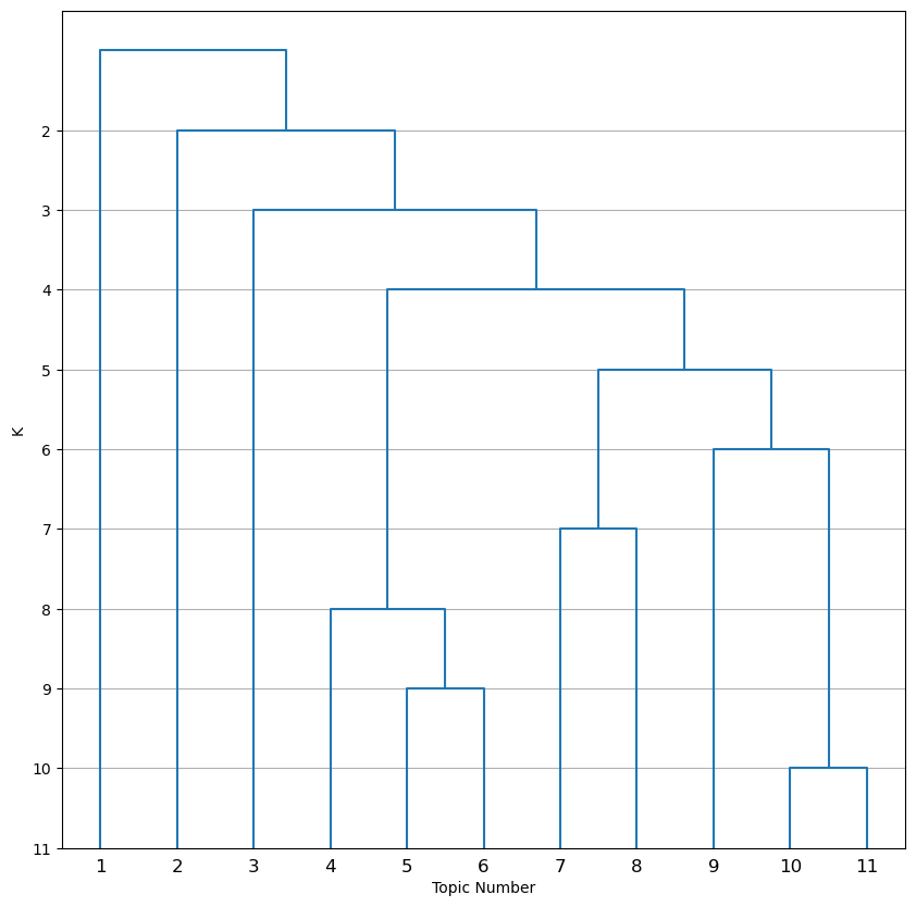
This image is a dendrogram showing how topics are hierarchically clustered and collapsed down to K=2. Next, open dendrogram_k11_distances.png.
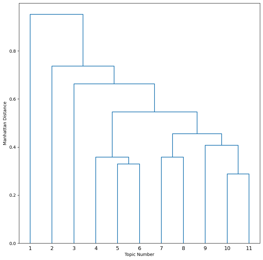
This dendrogram shows the same branching structure, but now the branch lengths correspond to the Manhattan distance between topics. Recall from Part I how topics 5 and 6 represented different portions of the hypothalamus. Note the relative position of these topics as sister branches in the dendogram.
Next, navigate to the deconvolution_k11 directory and open deconvolved_spots_k11.csv.
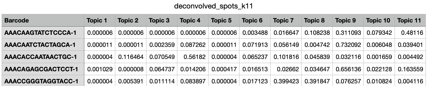
This file lists spots by row and different topics by column. Each cell represents the proportion of that spot assigned to that topic. In this way, you could use Loupe Browser to identify key spots of interest and pull their topic proportions from this file.
Finally, open the deconvolution_topic_features_k11.csv file.
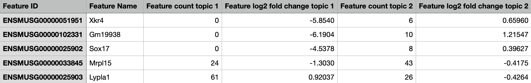
In this file, genes or features are listed as rows, and topics are listed by column; pseudocount and log2 fold change of features are provided for each topic. This file is meant to assist users in annotating topics with cell type.
- Read more about the algorithms underlying LDA-based spot deconvolution.
- Browse Space Ranger datasets
- Get started with Space Ranger
- Explore 10x Analysis Guides