- Learn how to navigate the Loupe Browser v7.0 (and later) UI using a Chromium Single Cell Gene Expression Flex lung cancer dataset and uncover new biological insights.
- Learn about the new and improved analysis features introduced in the v7.0 interface.
This tutorial demonstrates the navigation and interactive functionality of the Loupe Browser interface using a lung squamous cell carcinoma dataset. Three different types of lung tissue samples (untreated cancer, treated cancer, and normal tissue adjacent to cancer) were collected and sequenced. Learn more about the dataset by visiting the public datasets page.
Loupe Browser’s key interface components are shown here:
The workspace is centered around the View Panel in which single points representing cell barcodes are shown in a variety of projections. Each point represents a single barcode, the vast majority of which correspond to a single cell. The default projection is the t-SNE plot created by the Cell Ranger pipeline, though other projections are available (discussed below).
You can drag the mouse over the cells to reposition the plot and use the mouse wheel or trackpad to zoom in and out. Cluster labels appear as you move your mouse over the plot, which is useful for data that has a high number of precomputed clusters. Cells are colored by the active legend in the left panel (Mode Selector, discussed later).
The Projection type drop down controls the current projection in the View Panel. Most gene expression datasets will have the following projections available:
- t-SNE
- UMAP
- Feature Plot
Additional projections may be available, including:
- Feature Barcode-based t-SNE/UMAP plots
- Imported projections
- Projections derived from filtering and reclustering operations
Feature Plots
Loupe Browser's Feature Plot plots cell barcodes by the expression of one or two features. Feature Plots make it easy to threshold cell populations by expression, particularly for features with high dynamic range, such as cell surface markers. Features (genes in this example dataset) can be entered in the text boxes on the X and Y axes. These selectors also contain a control to switch the scale of the axis between linear and log scale.
Importing alternative projections
There are many scripts and community developed tools that can be used to generate different projections of the data, including but not limited to the following:
- Alternate clustering and projection algorithms, for example, trajectory analysis.
- Data filtered for unwanted artifacts, for example, dead or dying cells.
If you generate alternative projection coordinates from custom analysis, you can input that projection into Loupe Browser. To do this, click on the three vertical dots next to the projection type selector and Import custom projection (CSV file).
The CSV format for importing projections is as follows:
- A header is required.
- The first column contains barcodes that are at least a subset of the barcodes in the
.cloupefile. - The second column contains numbers that represent the X coordinates.
- The third column contains numbers that represent the Y coordinates.
In Loupe Browser v6.0 and later, you can also export the selected projection t-SNE or UMAP coordinates as a CSV file, including projections generated with the filtering and reclustering wizard.
Both t-SNE and UMAP projections are created by versions of Cell Ranger v3.1 and later.
As with previous versions of Loupe Browser, you can choose to open a different projection in a new window.
Split view enables you to view individual clusters from a projection adjacent to each other. Split view controls are in the ‘Split by’ dropdown menu located at the top of the graph. Click on the drop down, and select ‘disease state’ towards the bottom of the menu. It should be bold to indicate that it is the currently selected group.
You can see the distribution of the ten graph-based clusters in the three different disease states, Untreated Cancer, Treated Cancer, and Normal Adjacent Tissue:
Cluster labels in split view can be hidden by clicking on the hide cluster labels icon ![]() next to the ‘Split view’ drop down.
next to the ‘Split view’ drop down.
To exit Split view, click ‘x’ in the Split by menu.
The size of points on the graph can be adjusted using the ‘Projection settings’ ![]() drop down. Loupe Browser will auto-adjust point size to fit your window (default); unchecking the auto-adjust box allows you to change the size manually.
drop down. Loupe Browser will auto-adjust point size to fit your window (default); unchecking the auto-adjust box allows you to change the size manually.
The Mouse selector has three options from left to right:
- Pan
 : Move the image up and down, or left and right.
 - Lasso/rectangle selector
 : Select and label an image area with an irregular shape, or toggle the option to select and label a rectangular image area.
 - Draw selector
 : Select and label individual spots using a brush tool.
Export the scatter plot (UMAP, t-SNE, Feature Plot) in SVG (high resolution) or PNG (low resolution) format by clicking on the ‘Export’ drop down menu ![]() on the top right of the graph and selecting the format of interest. You can also export a list of barcodes and their (x,y) coordinates in CSV format via this drop down.
on the top right of the graph and selecting the format of interest. You can also export a list of barcodes and their (x,y) coordinates in CSV format via this drop down.
Options to zoom in on specific regions of the graph are provided at the bottom left of the graph. Clicking on the zoom icon brings up a sliding scale ![]() that can be adjusted with your mouse. Click on the graph and drag your mouse cursor to adjust the view region. The autoscale icon
that can be adjusted with your mouse. Click on the graph and drag your mouse cursor to adjust the view region. The autoscale icon ![]() can be used to scale the graph back to fit the current screen dimensions. Autoscale is also useful for recentering the graph after pan exploration.
can be used to scale the graph back to fit the current screen dimensions. Autoscale is also useful for recentering the graph after pan exploration.
The left panel of the workspace is the Mode Selector. Switching between modes applies mode-specific coloring to the graph (on the right).
You can hide the mode selector options by clicking on the hide UI button ![]() located next to the save icon.
located next to the save icon.
There are three ways to display data clusters:
- Graph-Based Clustering
- K-means Clustering from K=1-10
- Any number of custom-created groups and their corresponding cluster names.
The custom groups for this example dataset are shown in the image:
Loupe Browser extracts custom groups from the aggregation CSV that was used to run cellranger aggr. Custom groups can also be created using the Loupe Browser interface or imported as a CSV (upload icon ![]() next to ‘+ Create a new group’). An example CSV file used to create a custom group called "Clonotype" is provided below. The first column lists the barcodes of interest, while the second column, labeled "Clonotypes," specifies the group each barcode belongs to. The header of the second column will appear as the group name in Loupe Browser.
next to ‘+ Create a new group’). An example CSV file used to create a custom group called "Clonotype" is provided below. The first column lists the barcodes of interest, while the second column, labeled "Clonotypes," specifies the group each barcode belongs to. The header of the second column will appear as the group name in Loupe Browser.
Barcode,Clonotype
AAACATACGGTACT-1,Clonotype_1
AAACATTGCTCGCT-1,Clonotype_1
AAACATTGGCGATT-1,Clonotype_2
AAACCGTGTGCCTC-1,Clonotype_2
AAACGCTGACCTCC-1,Clonotype_2
Custom group names can be edited at any time. While Cell Ranger-generated group names are not editable, cluster names and colors within all groups (Cell Ranger-generated groups and custom groups) are editable.
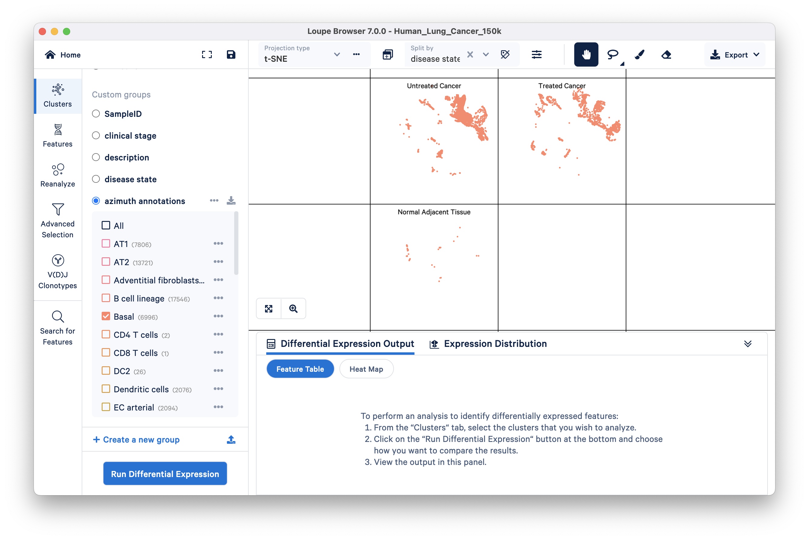
This example comes with a pre-annotated group called 'azimuth annotations'. The azimuth annotations group contains canonical lung cell type annotations that were determined using the automated reference-based annotation tool Azimuth. Selecting this category reveals a list of cell types (clusters) and colors the graph by clusters in this category. You can look at all the clusters at once by selecting ‘all’ (default) or check the cell types of interest.
Here, you are looking at the distribution of basal cells split by the three different disease states: Untreated Cancer, Treated Cancer, and Normal Adjacent Tissue. Basal cells are thought to give rise to squamous cell lung carcinoma. We can see that there are fewer barcodes annotated as basal cells in the Normal Adjacent Tissue group compared to the two cancer groups.
The Cluster Mode panel has a 'Run Differential Expression' option that enables you to find genes that uniquely characterize individual clusters. These options are available:
- Compare selected clusters to entire dataset: For each selected cluster in a group, identify features that are upregulated in a given cluster relative to all other clusters in the dataset and find the features that distinguish that cluster from every other cluster in the dataset.
- Compare selected clusters: For each checked cluster or group, find the features that distinguish that cluster from the other currently checked clusters in that group.
- Compare selected clusters across multiple samples: For the selected groups, find features that are differentially expressed between two conditions using a pseudo-bulk calculation.
Loupe Browser uses the same statistical method as Cell Ranger (source code available) to calculate differential gene expression in all the above cases. The mean expression between groups of cells is calculated using an exact negative binomial test (sSeq method). For large UMI counts, the algorithm switches to the fast asymptotic negative binomial test used in edgeR. Visit Cell Ranger's Gene Expression agorithm page for details.
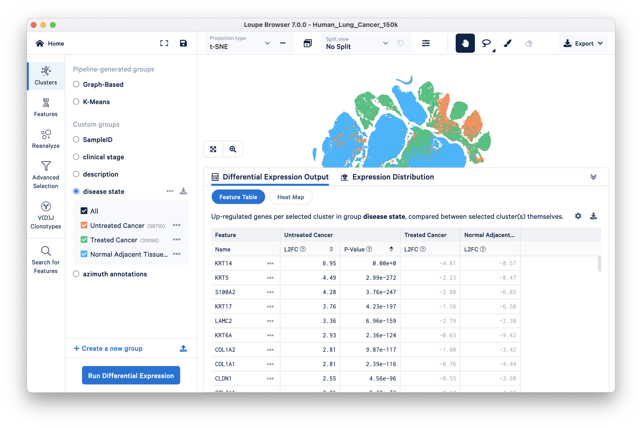
We will find genes that distinguish the Untreated Cancer from the rest of the dataset (Treated Cancer and Normal Adjacent Tissue). Select the disease state group and click 'Run Differential Expression'. Next, click on the 'compare selected cluster(s)' drop down and select the 'To entire dataset' option. Keep Feature type as Gene (the only available option) and start the analysis. The pop up window disappears when you click 'Start analysis' and the results of differential expression (DE) analysis will take a few seconds to appear in the Data Panel of the original Loupe Browser window.
The Differential Expression Output tab is selected by default. This tab has the option to view the results of DE analysis either as a Feature Table (default) or a Heat Map.
Feature Table: significant gene information in a tabular view. For each cluster, you can view the most significantly upregulated genes per cluster by p-value or L2FC (Log2 fold change) values. Click the setting button ![]() on the top right of the Data Panel for more options to filter by.
on the top right of the Data Panel for more options to filter by.
In this lung cancer dataset, basal cell markers (e.g., KRT14, KRT5, S100A2, KRT17) are upregulated in the tumor group compared to the other two groups. As previously mentioned, squamous cell carcinoma originates from basal cells. However, at this analytical level, it is not yet clear whether this observation suggests a higher abundance of basal cells in the Untreated Cancer group or if it indicates a cancerous phenotype within the basal cell type. To gain more insight, we can investigate this question further through subsequent analyses involving multi-sample comparisons (described later in the tutorial).
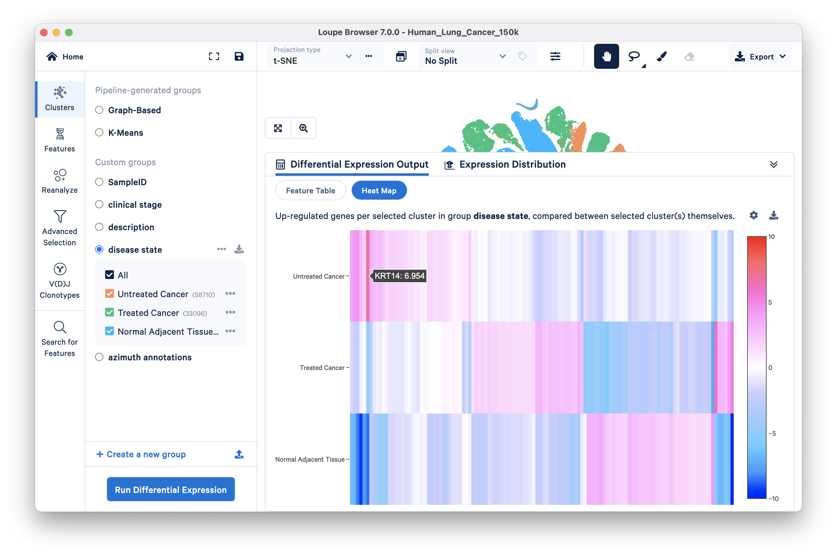
Heatmap: The heatmap takes the top n genes and hierarchically clusters them. The number of genes (n) varies based on the number of clusters in the analysis (discussed in this Knowledge Base article). Each column represents the level of expression of a significant feature and each row represents a cluster. Grid cells are colored by a gene's L2FC in its cluster row, compared to the other clusters. Hovering over the columns will show the names of the features represented in each column.
In the previous comparison, including the Normal Adjacent Tissue group may have masked smaller differences between Untreated Cancer and Treated Cancer. To identify what distinguishes the two cancer groups from each other, we can identify significant features distinguishing just these two groups by excluding Normal Adjacent Tissue.
Uncheck the Normal Adjacent Tissue group, and run the same differential expression analysis as before:
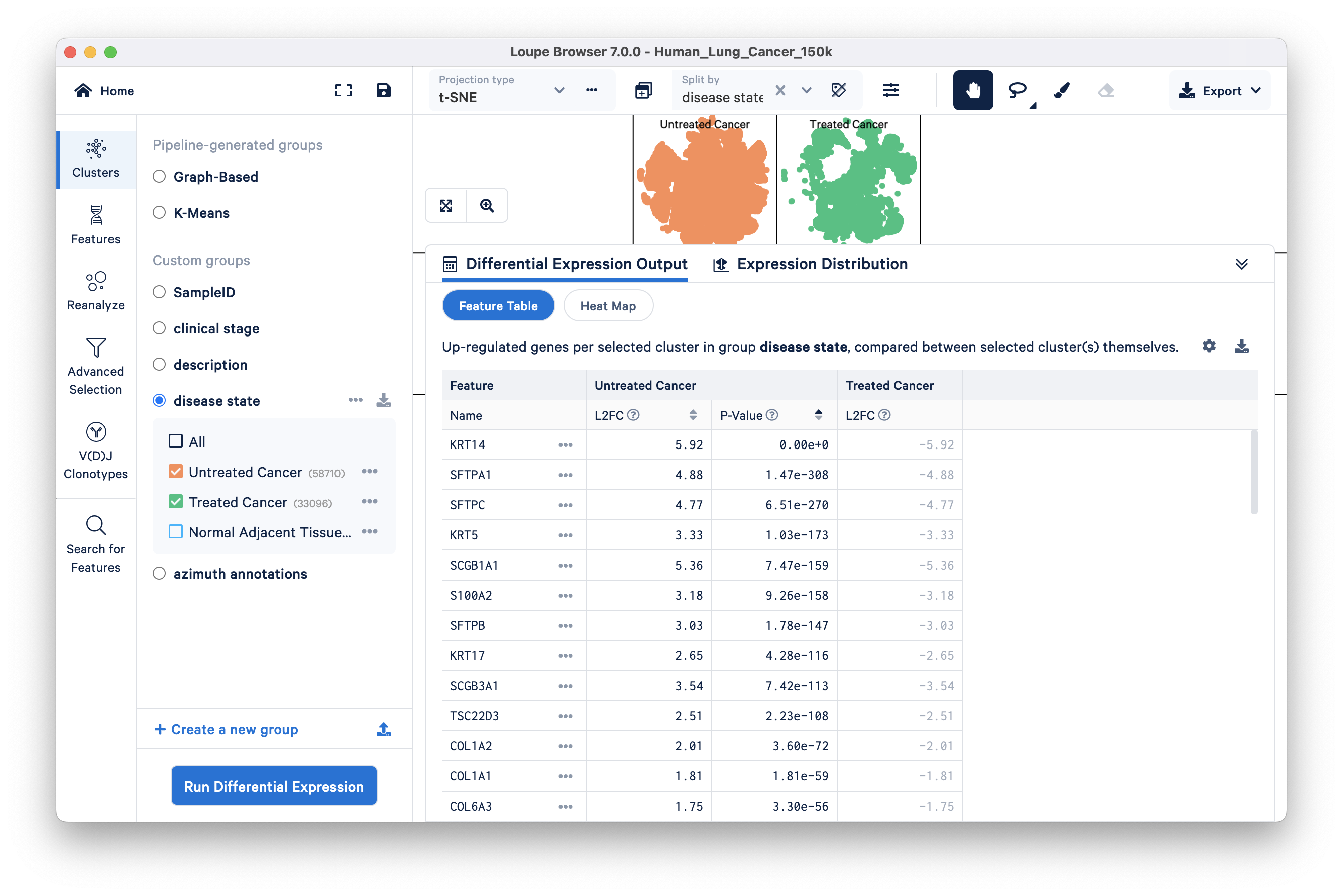
Click on the Treated Cancer column to see the top upregulated genes in that group relative to Untreated Cancer. Among the most upregulated genes, CEACAM6 is notable and is known to play a role in CD8+ T cell responses, which is a positive indicator for lung cancer treatment. Additionally, it is not surprising to find CES1 upregulated in the "Treated Cancer" group, as CES1 is a drug-metabolizing enzyme, and its upregulation may be associated with the metabolism or processing of drugs used in cancer treatment.
Importing a Feature list
We demo the Features functionality with this pre-made Feature List for you to import into Loupe Browser.
The CSV looks like this:
| List | Name |
|---|---|
| Immune | CD53 |
| Epithelial | PIGR |
| Epithelial | CYB5A |
| Epithelial | MUC1 |
| Endothelial | CLDN5 |
| Endothelial | VWF |
| Stroma | TPM2 |
| Stroma | DCN |
| Stroma | LUM |
| Stroma | COL1A2 |
| Basal | KRT5 |
| Basal | KRT17 |
| Basal | S100A2 |
The first column is the group or type of feature, whereas the second column is the name of the feature (gene) corresponding to that group. There are five groups of cell type markers (Immune, Epithelial, Endothelial, Stromal, and Basal), and four out of five of these groups have multiple features.
To import a feature list, click the upload button located at the bottom of the Features mode selector and upload the 157k_21_NSCLC_multiplex/157k_21_NSCLC_multiplex_Features.csv:
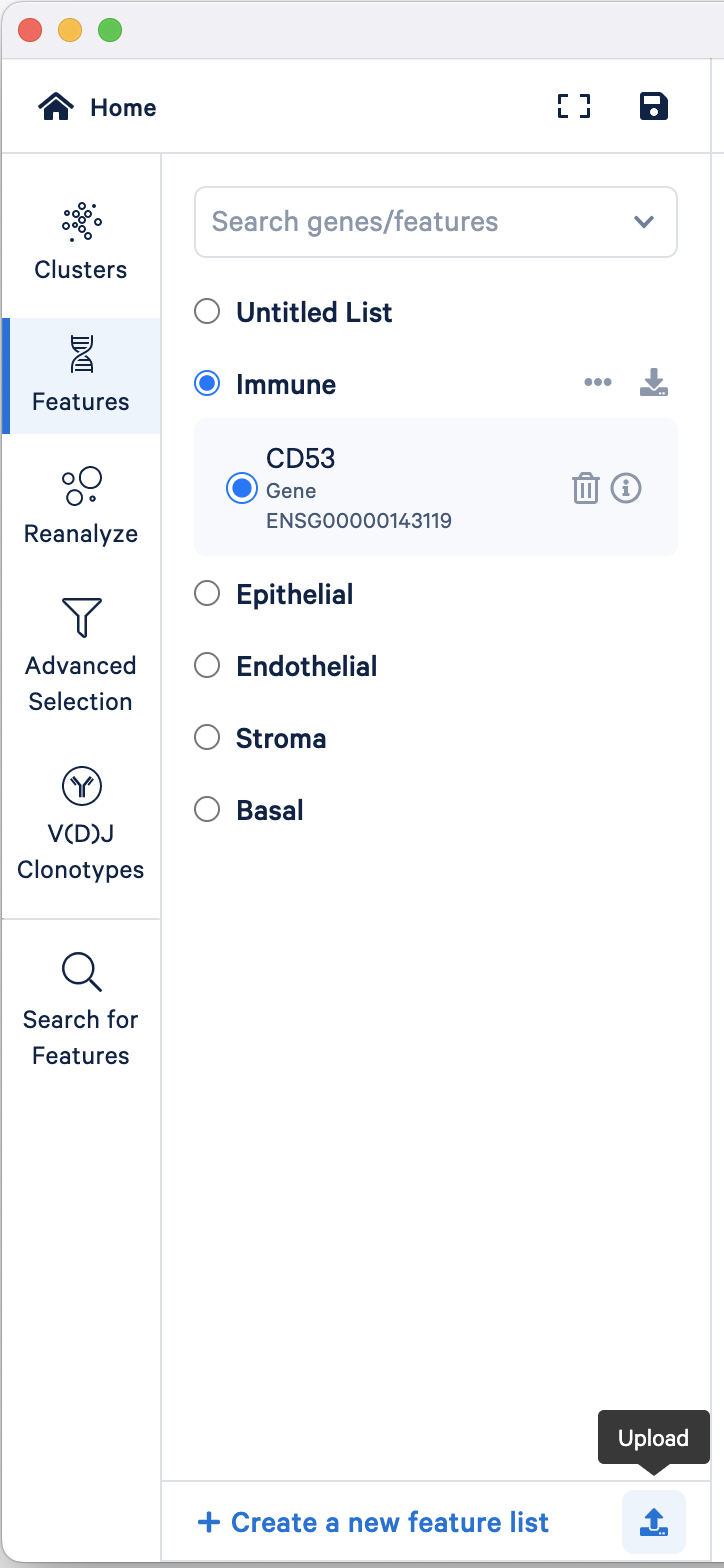
By default, each group (with multiple features) has the "Combine all below" option selected. However, you can view the expression patterns of individual features by selecting that feature.
There are several options (right) that control how the data are visualized based on the feature list.
The Scale value drop down sets which scale value to display and has the options: Linear, Log2, and LogNorm.
- When Linear is chosen, actual UMI counts are rendered in the View Panel, without any normalization.
- Log2 is the default setting and displays log2-transformed rendering of UMI counts in the View panel.
- Selecting LogNorm as the scale enables viewing of feature expression normalized by UMI count (for single cell and spatial datasets) or cut site count (for ATAC datasets). The log-normalization method is the same as methods used in Seurat and Scanpy, with quantitative expression computed as follows:
where the barcode count is the total number of UMIs or cut sites associated with the barcode. The relative expression ratio is multiplied by 10,000 to shift the relative expression distribution above the constant introduced by the log1p operation.
The Combination drop down (only available for groups with multiple features) has options on how to combine values when there are multiple features in the Active Feature List and has options:
- Feature Max: Displays the maximum expression value of the features in the list when at least one feature is expressed. This is the default selection when you import a feature list.
- Feature Min: Displays the minimum expression value of the features in the list when all features are expressed.
- Feature Sum: Displays the summed expression of all features in the list.
- Feature Avg: Displays the average expression of features in the list.
- UMI Count: Displays the total UMI counts of all features in every cell barcode.
Select the Basal feature and split the view by azimuth annotation:
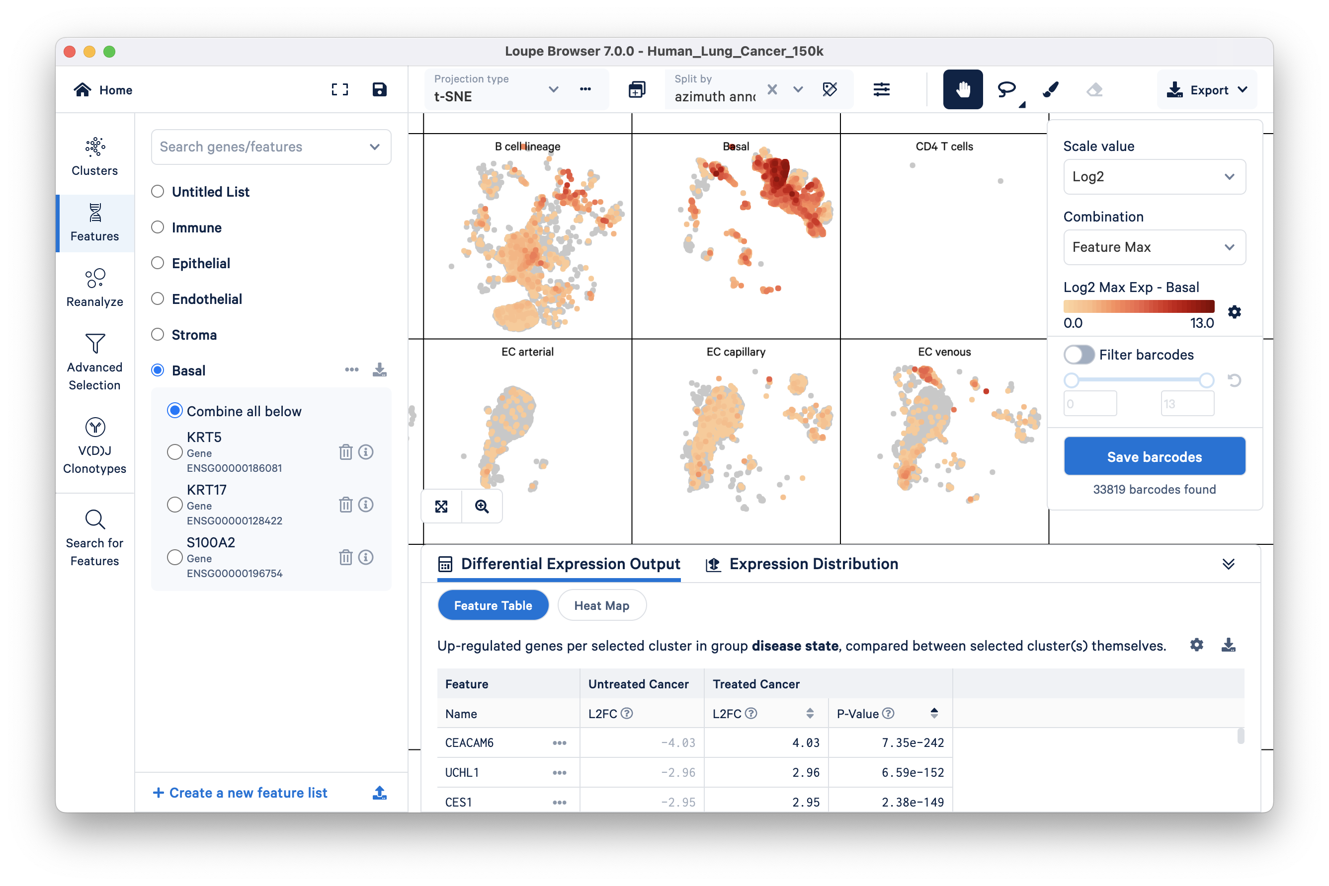
This view allows you to quickly compare your imported basal markers with the pre-annotated cell types; you can see here that basal cell markers are highly expressed in the pre-annotated basal cells group.
Click on a different feature in your imported list to view the distribution of that feature. Please note that any customizations in the view settings from one feature do not transfer over.
Searching for Features manually
It is also easy to create a custom feature list via the search option in Features mode. We will add a few more features to the basal group: KRT15, SFN, and IGFBP2. Make sure the Basal group is selected, then search the first gene feature, KRT15, by typing in the ‘Search genes/features’ box at the top. Clicking on the gene name that appears in the search result should add that gene to the selected feature group. Repeat this for SFN and IGFBP2.
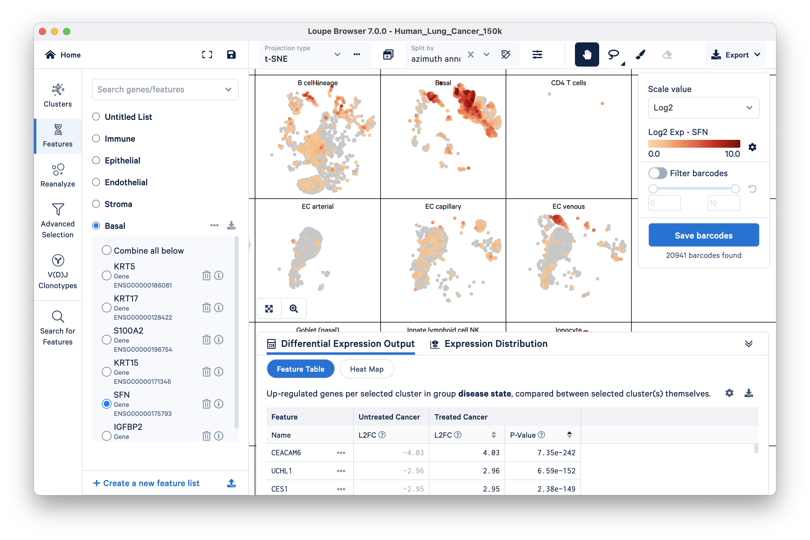
As you can see, these additional basal cell marker genes are also highly expressed in the Basal cell cluster.
Loupe Browser v7.0 and later allows users to find features that are differentially expressed in two experimental conditions using a pseudo-bulk calculation. Loupe Browser's algorithm reads the entire gene expression count matrix. For every cluster, a new matrix is made in which each column is the sum of all barcodes in that sample. Finally, sSeq is run on each of these compacted matrices; the algorithm is identical to that used by Cell Ranger.
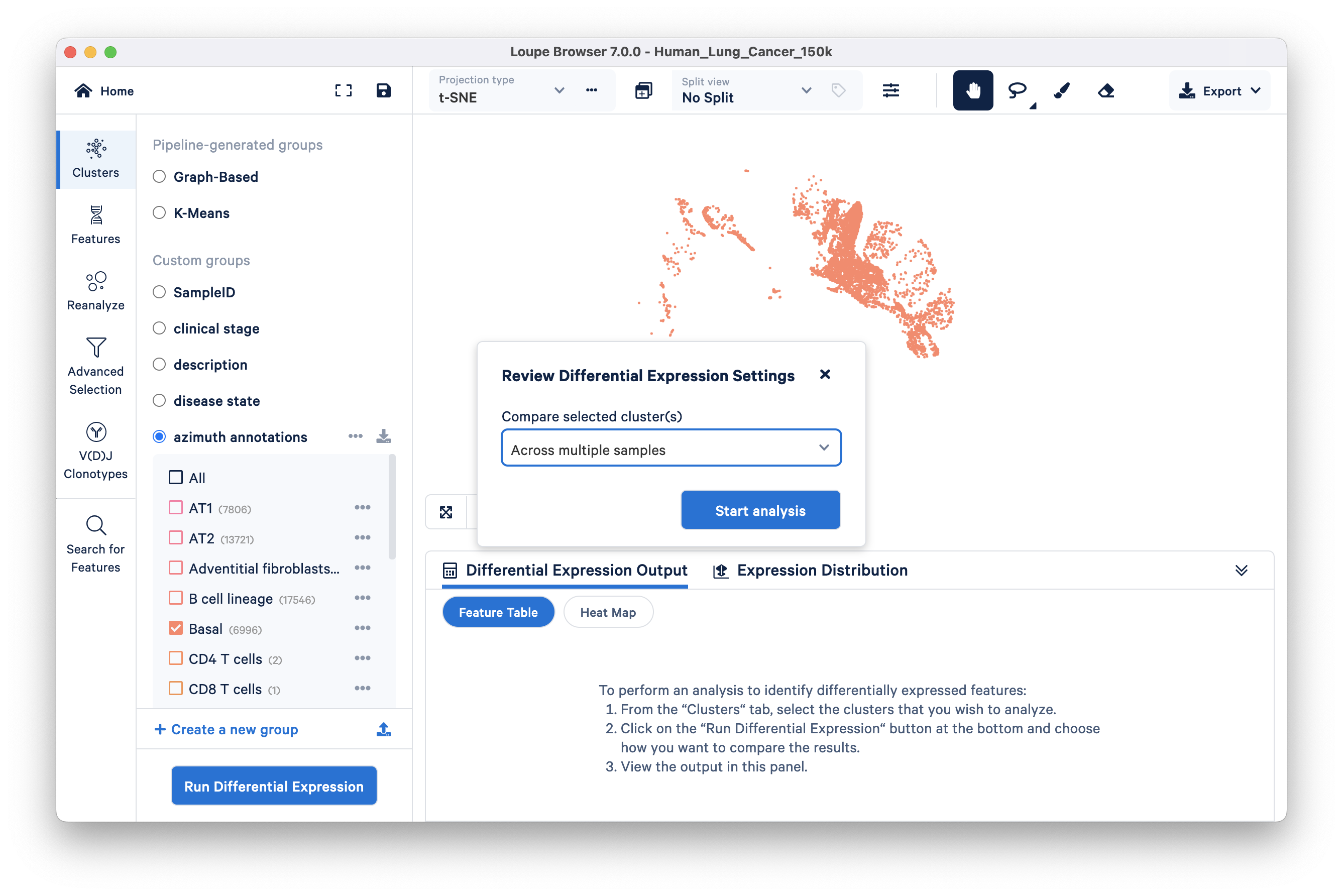
We saw earlier in this tutorial that many basal cell markers were upregulated in the Untreated Cancer group. Basal cells are known to be the origin cells in lung squamous cell carcinomas. Therefore, it is worth digging deeper into genes that distinguish the basal cells of treated versus untreated patients.
We will run a multi-sample differential gene expression analysis to identify up and down-regulated genes in the basal cell type of treated versus untreated patient samples.
Click the Run Differential Expression button, select the ‘Across multiple samples’ option from the Compare selected clusters drop down, and start analysis:
This opens a new Loupe window describing how to use the multi-sample differential gene expression wizard:
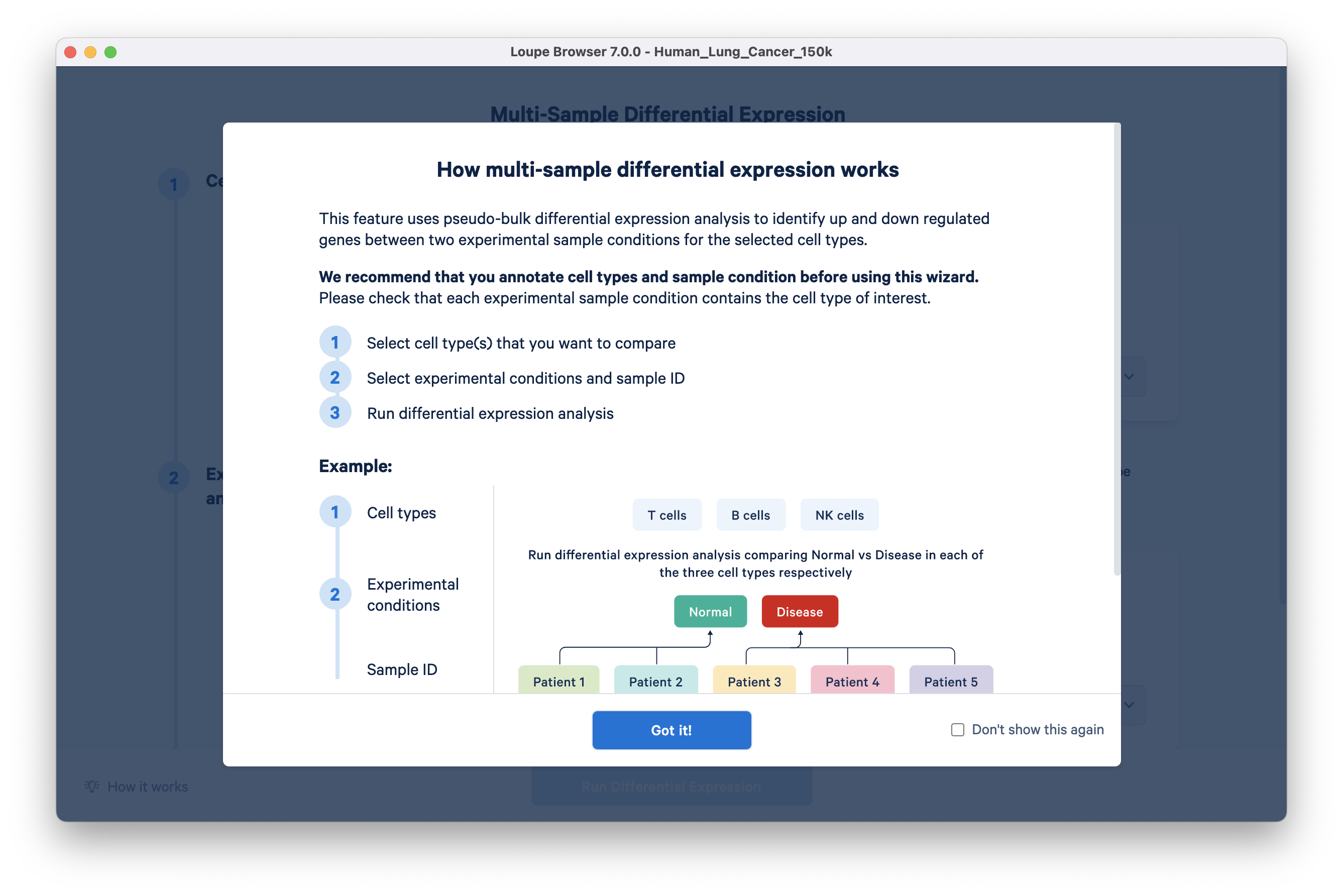
Step 1: In the Cell Types section, choose azimuth annotations in the ‘From category’ dropdown menu. All clusters in this category are auto-populated in the Cell Types tab. Keep the Basal cluster, and delete the rest of the clusters in this list. A faster way to do this is by clicking the "X" to delete all and then selecting "Basal" from the drop down.
Step 2: In Experimental conditions, select ‘disease state’ in the ‘From category’ drop down. Select Untreated Cancer as condition A and Treated Cancer as condition B.
Step 3: In the sample ID section, select SampleID in the ‘From category’ drop down. Conditions A and B are auto-populated by the wizard:
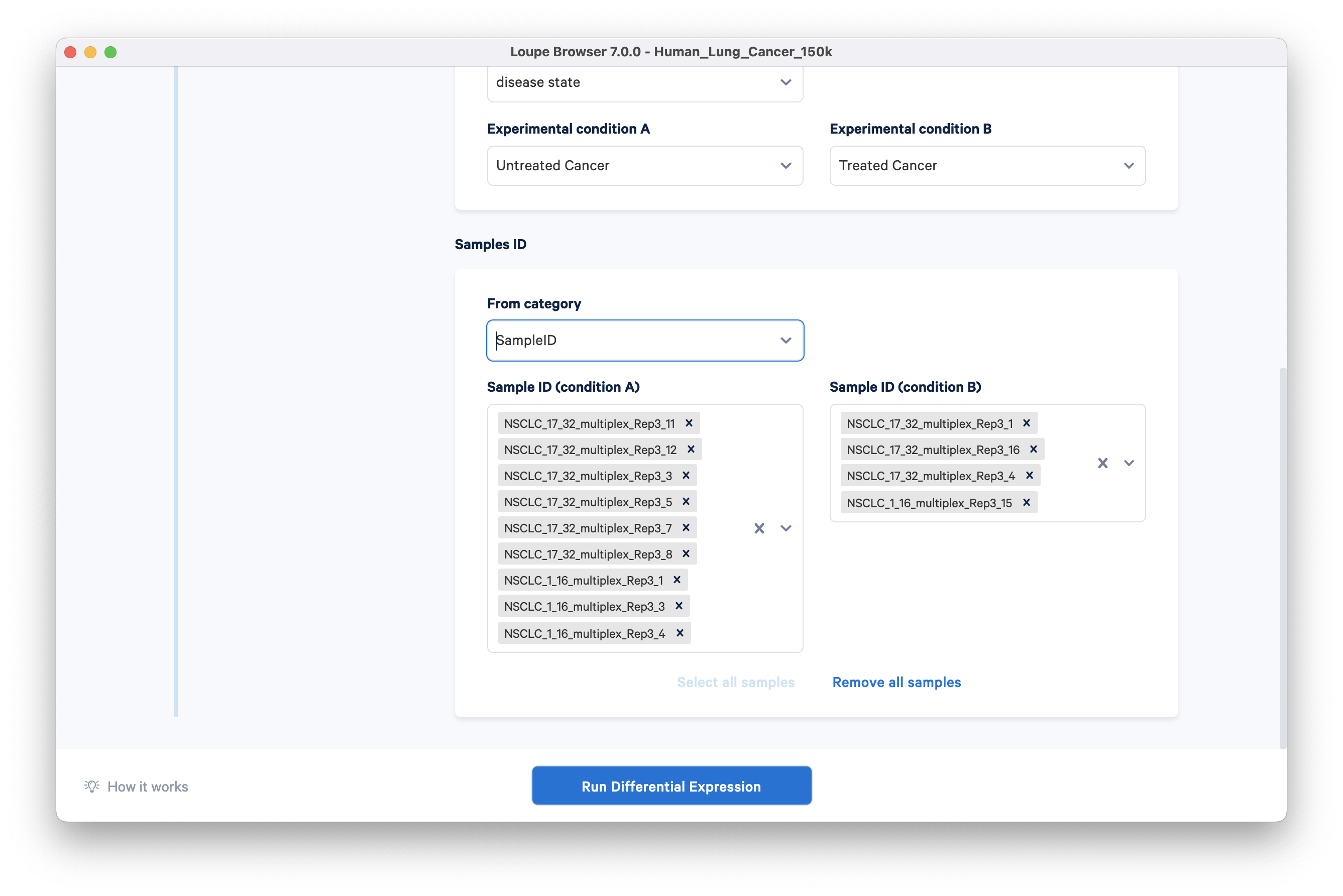
Please note that if a particular sample does not have any barcodes assigned to one of the cell types selected in Step 1, it will be highlighted yellow. Analysis cannot proceed until either the cell type or the sample is deleted.
Finally, click Run Differential Expression.
Results are displayed in the primary Loupe Browser window.
The Feature table is shown here. Look at the top three upregulated genes in the Untreated Cancer (Condition A) versus Treated Cancer (Condition B):
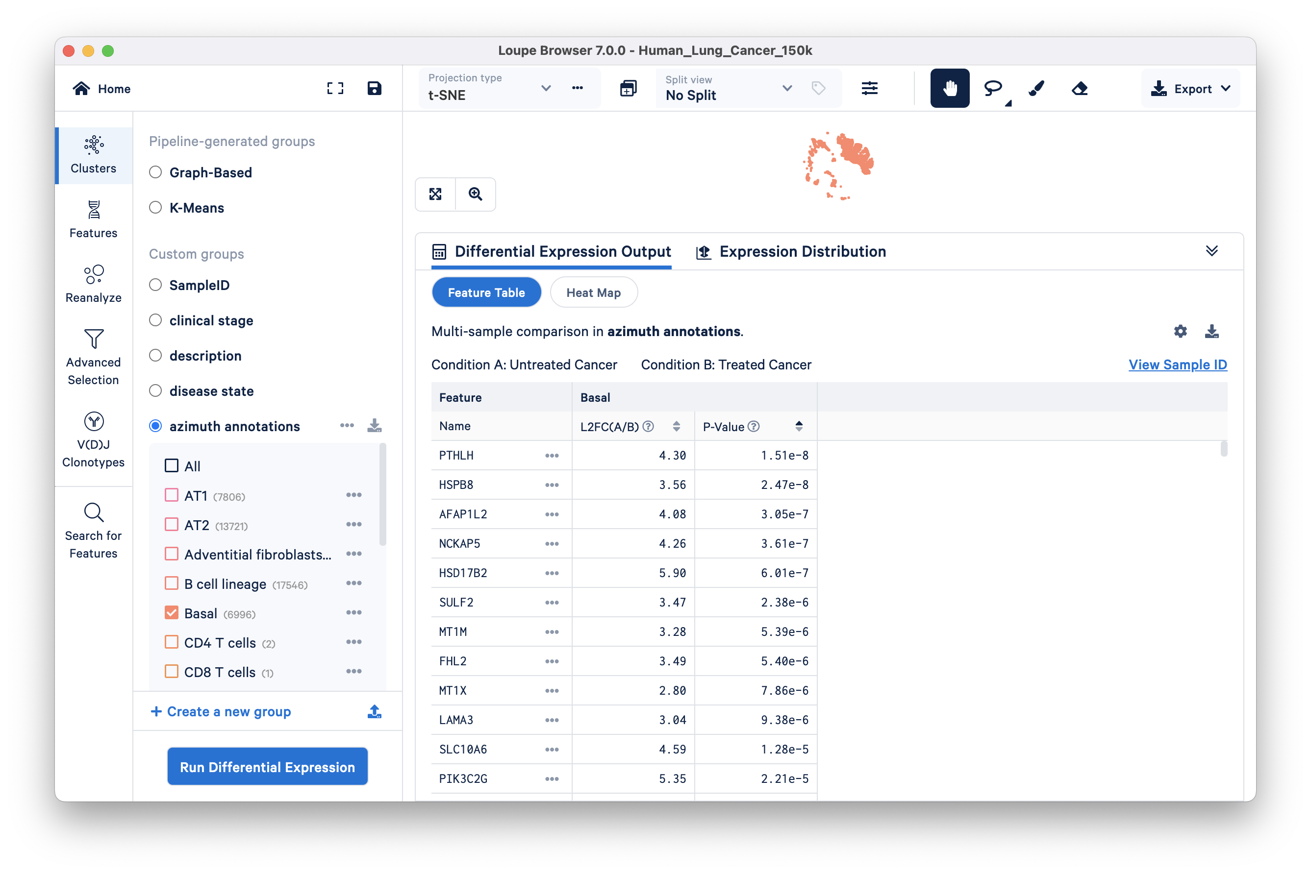
- PTHLH, is secreted by certain kinds of squamous-cell lung cancer cells
- NCKAP5: differentially expressed in non-small cell lung cancer and associated with patient survival
- SULF2: encodes heparan sulfate 6-O-endosulfatase, an enzyme that promotes the growth and metastasis of solid tumors. Similarly, some of the interesting downregulated genes are discussed below (displayed in the Feature Table via changing the Filter feature by setting):
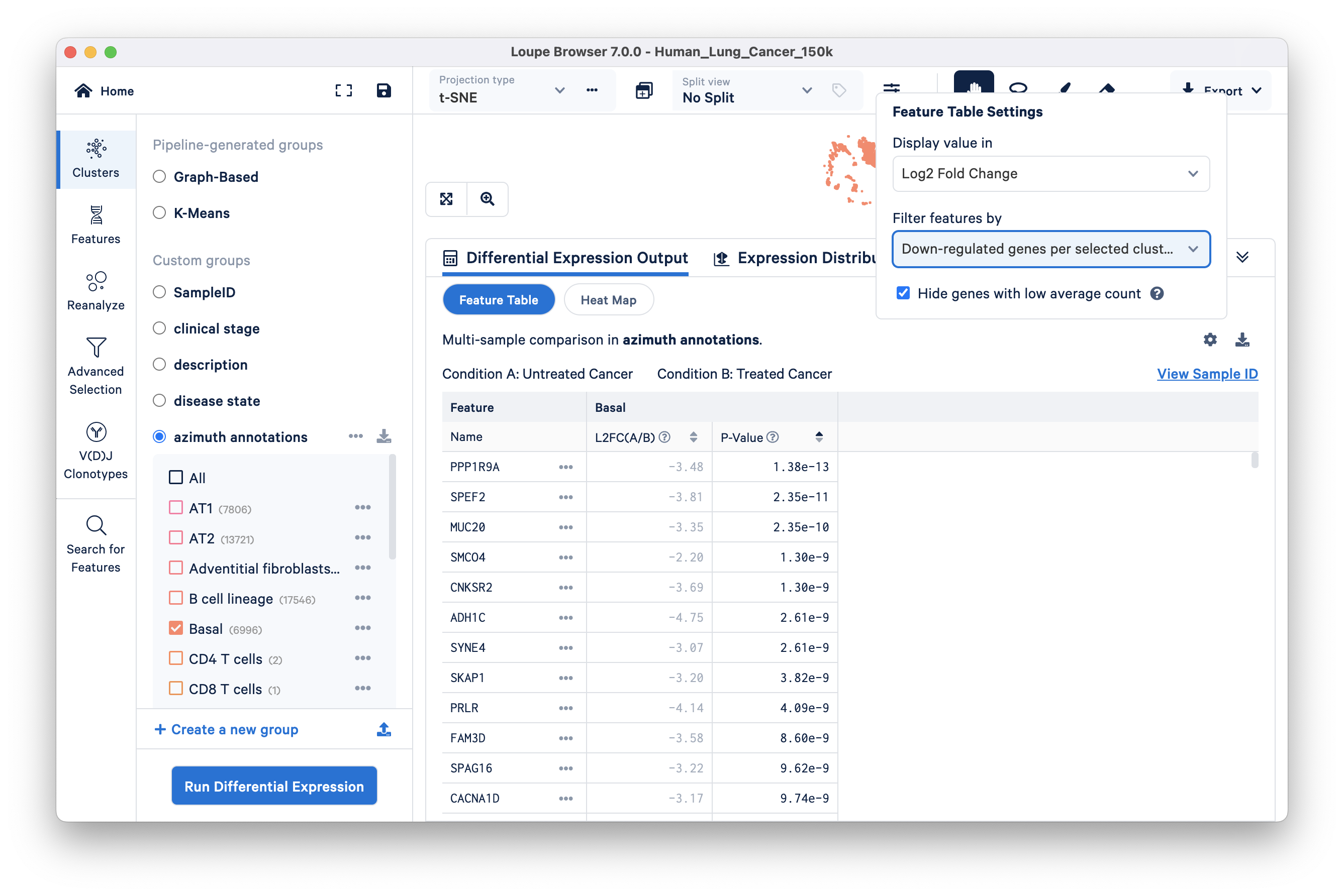
PPP1R9A: PP1s are related to a poor prognosis in numerous cancers including lung cancers.
MUC20: is a poor prognosis marker
PRLR: has been shown to confer resistance against chemotherapeutic agents including docetaxel, doxorubicin, and cisplatin
In Loupe Browser v7.0, the reclustering workflow is available in the Mode selector panel as Reanalyze. Clicking on the Reanalyze button opens a new window. The workflow remains similar to that available in Loupe Browser v6.5.
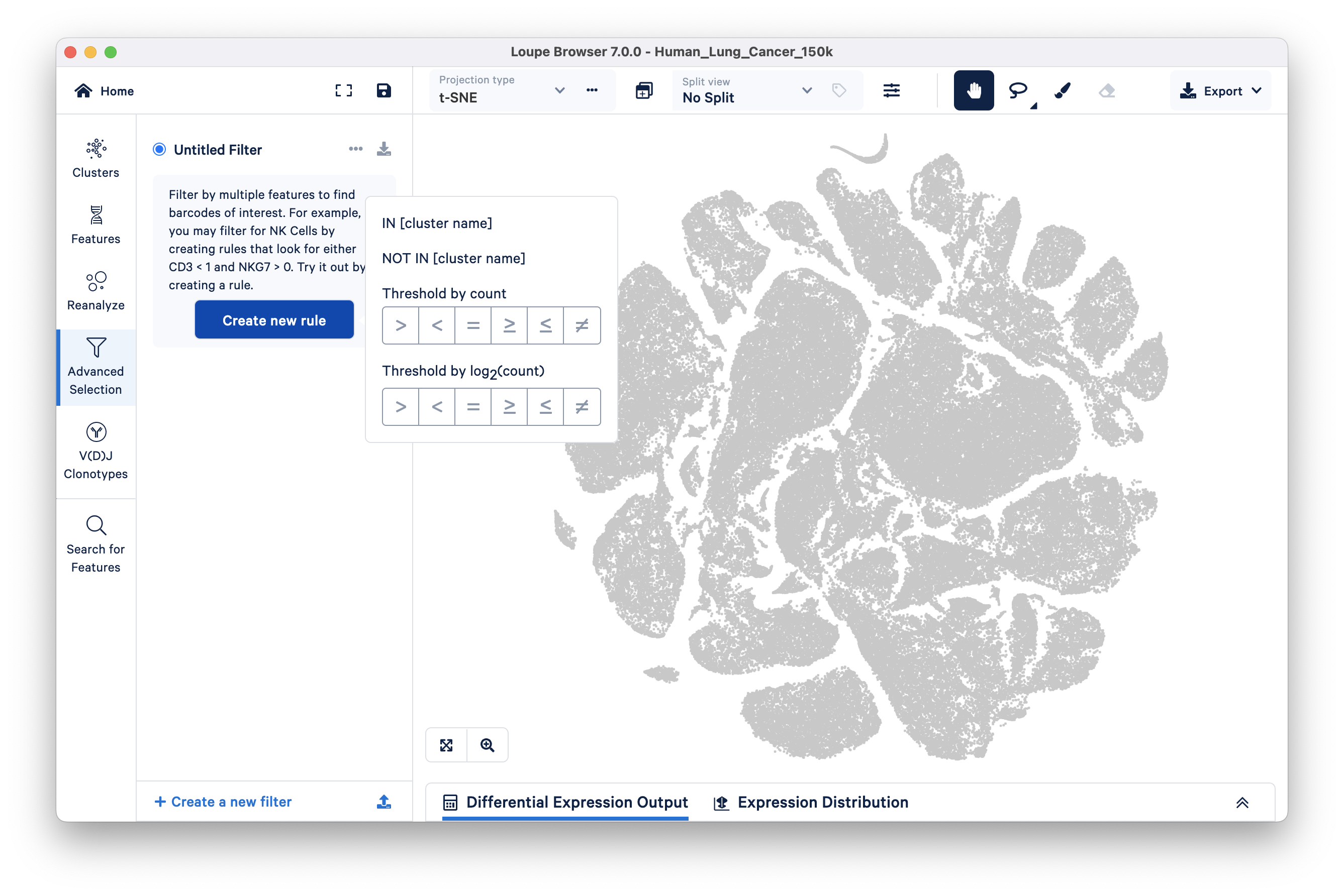
The Filters options available in Loupe Cell Browser v3.1 and Loupe Browser v4.0 (and later) are now available under the Advanced Selection button of the Model selector panel.
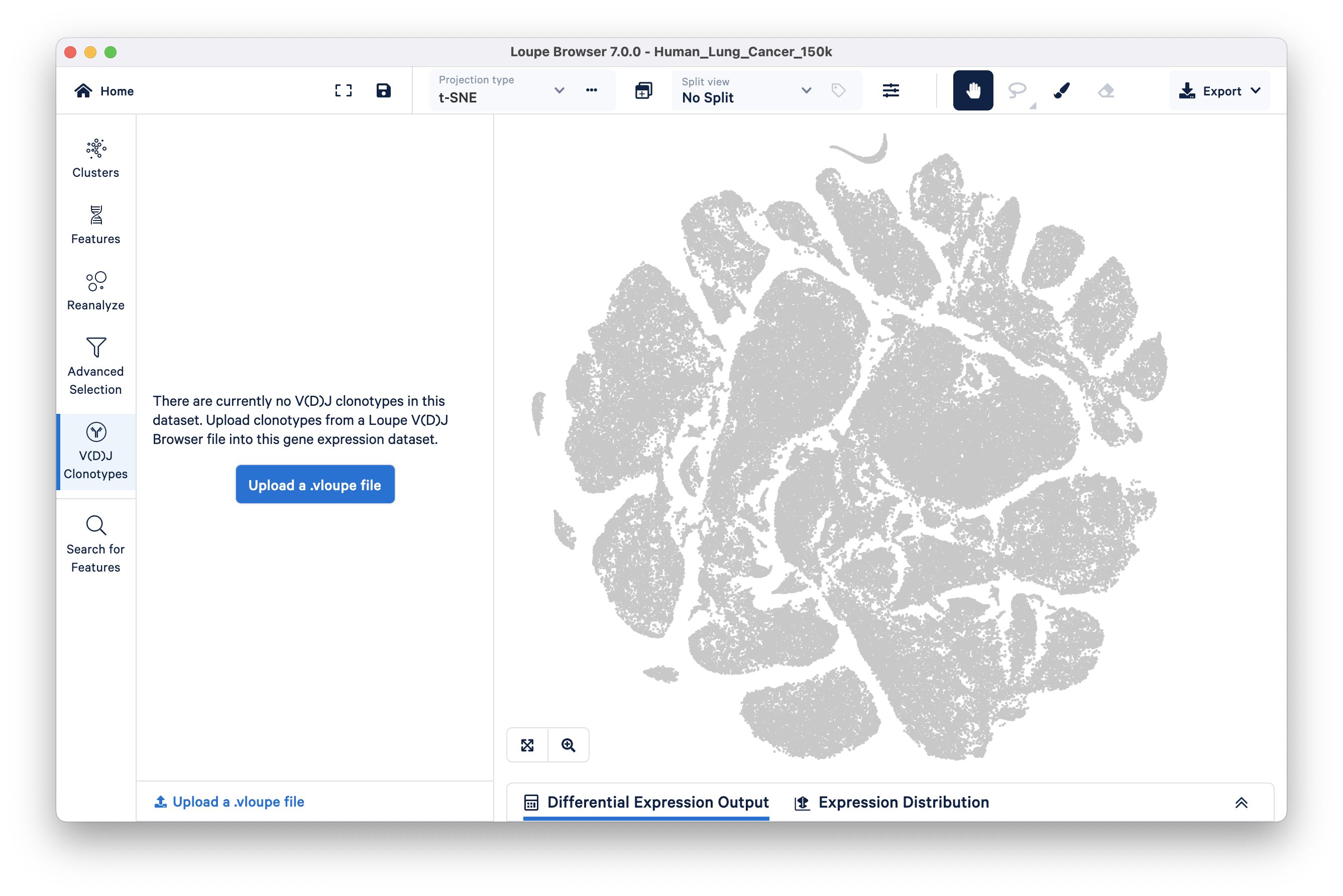
If your dataset includes a VDJ-T or VDJ-B library (with or without Antigen Capture) you may wish to import the corresponding .vloupe file to explore clonotypes within gene expression clusters.
To import a .vloupe file, click on the V(D)J Clonotypes button in the Mode selector panel, then click Upload a .vloupe file.
The graph changes to highlight (in blue) only T or B cell barcodes.
Click on a specific clonotype in the list on the left to further highlight that clonotype in the View panel.
Filter options in the Loupe Browser v7.0 interface are similar to those available in earlier versions. However, these options have moved to the Mode Selector on the left side.
The ‘Save barcodes’ button allows you to save V(D)J clonotype barcodes to new or existing clusters for further investigation in Loupe Browser.
Please visit the Integrated V(D)J and Gene Expression Analysis in Loupe Browser tutorial to downloadable example .cloupe and .vloupe files and try them out in the new interface.
Use the save icon ![]() to save all customizations to your
to save all customizations to your .cloupe file.
You may also wish to rewrite to a new .cloupe file by clicking File -> Save as -> provide a new file name -> save.