Note: 10x Genomics does not provide support for community-developed tools and makes no guarantees regarding their function or performance. Please contact tool developers with any questions. If you have feedback about Analysis Guides, please email analysis-guides@10xgenomics.com.
The Xenium workflow is nondestructive and enables researchers to derive additional information from the identical tissue section, including H&E and immunofluorescence (IF). The supplemental imaging must use a different microscope system. To leverage the additional spatial image data in relation to Xenium cell and transcript coordinates, the image must be registered to Xenium data coordinates. This tutorial illustrates tissue image registration using an H&E image and the Xenium DAPI image for the same tissue section.
Software and data download links are in section 1. The tutorial provides some background on the algorithms (section 2), illustrates how to perform a simple image registration (section 3; results shown in GIF above) and shows how to visually inspect the result (section 4). For H&E images with proper image preprocessing, the linear transform in section 3 should suffice for registration. The tutorial provides some advanced discussion on extracting keypoint coordinates (section 5) and elastic registration (section 6) that may be of interest to those coding custom solutions and for other contexts, e.g. registering an adjacent tissue slice image.
- Software and data
- Background
- H&E-to-DAPI image registration with SIFT
- Check registration effectiveness
- (Advanced) Extract keypoints or landmarks
- (Advanced) H&E-to-DAPI image registration with bUnwarpJ
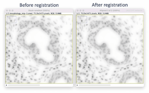
The resulting registered H&E image’s hematoxylin features will approximately match the DAPI image features in relative XY space. We can then use the registered H&E image in downstream secondary analyses to correlate regions to cells, e.g. stLearn’s spatial trajectories inference. The simple registration does not correct for any differences in optics in the two microscope systems, nor account for stitching artifacts. Therefore, results may or may not be suitable for more refined analyses, e.g. to correlate Xenium transcripts to cells derived from H&E-based cell segmentation.
- See the article What are the Xenium image scale factors? for how the Xenium cell feature matrix and transcripts coordinates relate to the Xenium image TIFF series and for Python code examples including code to resample and plot transcripts overlaid on the DAPI image.
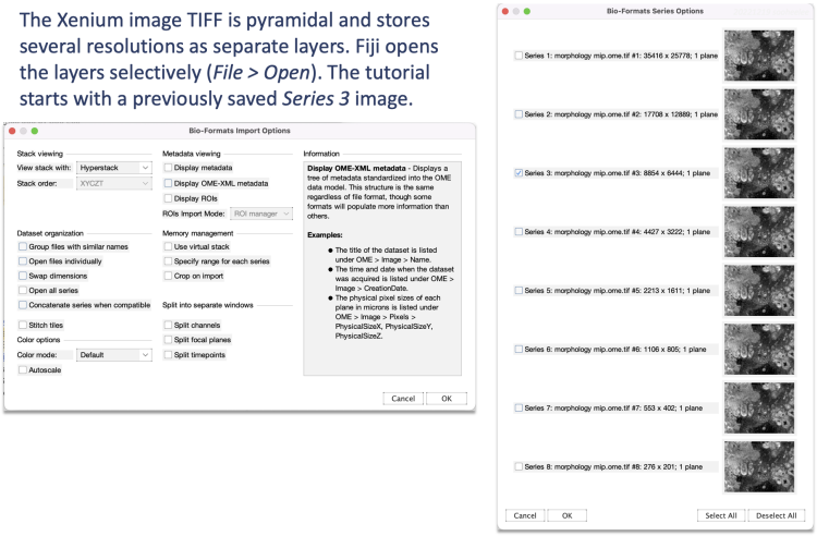
The publicly available Xenium human breast cancer dataset comes with supplemental H&E and IF images. In this tutorial, we use Replicate 1's Series 3 DAPI image^ and a previously resized and cropped H&E image for simplicity.
Download the preprocessed, full-sized H&E image morphology_he-shlee.png, the single-layer DAPI image morphology_mip.ome.3.invert.tif (start with step 3.2); the subset H&E image used in section 6 tiny-he-lens.tiff and the corresponding DAPI image tiny-mip-inverted.tif. The resulting registered H&E image from section 3 is he-registered-to-dapi-shlee.tif.
The tutorial uses Python v3.8.2 and desktop software Fiji (ImageJ) v2.9.0/1.53t. The anaconda download from https://www.anaconda.com/products/distribution should install most dependent Python packages. Fiji is downloadable from https://imagej.net/software/fiji/downloads. Other image registration approaches exist, e.g. Napari plugins and custom code solutions. We illustrate with Fiji due to its compatibility with Windows, MacOS and Linux operating systems, a graphical user interface (GUI), and extensive documentation and support.
- For an introduction to Fiji (ImageJ), see the beginning of Testing microscope image compatibility with Space Ranger.
- To increase the memory Fiji can use, go to Edit > Options > Memory and Threads and set maximum memory to 75% of available physical memory. If memory is still limiting, check Memory management > Use virtual stack.
The tutorial does not cover IF image registration. The Xenium public human breast cancer dataset Replicate 1 includes an IF image stack, where the DAPI layer is channel 3, for testing.
- Registration depends on feature matching. To enable IF stain registration to Xenium’s DAPI image, image a DAPI stain in the same session as the IF stain(s) to produce a multi layer TIFF. The tissue slice may need a fresh DAPI stain, as the Xenium instrument workflow greatly reduces the instrument DAPI stain signal. Moreover, residual DAPI stain signal precludes use of the DAPI channel for other epitope detection.
Future 10x Xenium software may incorporate image registration capabilities. Please check the Xenium software documentation at /support/in-situ-gene-expression for updates or inquire at support@10xgenomics.com.
The documentation at https://imagej.net/imaging/registration introduces image registration and summarizes Fiji registration plugins. This article illustrates the use of the following plugins.
- Linear Stack Alignment with SIFT (Plugins > Registration > Linear Stack Alignment with SIFT). SIFT stands for Scale Invariant Feature Transform and extracts features from images. The plugin uses the features common across images to align the images in a stack quickly using only linear transformations. The plugin offers four linear models.
- Translation transforms up, down, left and right
- Rigid (Euclidean) transforms add rotation
- Similarity transforms add uniform or isotropic scaling that adds equal scaling in all directions.
- Affine transforms add shearing
Of these, affine gives the most degrees of freedom as illustrated here. Section [3] illustrates SIFT registration using the affine model.
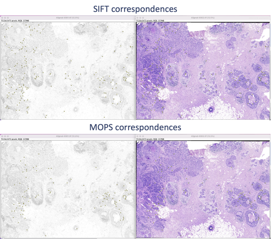
- Feature Extraction (Plugins > Feature Extraction). Automatic feature extraction that results in keypoints, aka landmarks, in both images as detailed at https://imagej.net/plugins/feature-extraction. Section [5] illustrates using SIFT and MOPS correspondences. Details on Multi-Scale Oriented Patches are here and here.
- bUnwarpJ (Plugins > Registration > bUnwarpJ) for elastic (non-rigid) image registration. bUnwarpJ elastically deforms the target image to look as similar as possible to the source image as explained at https://imagej.net/plugins/bunwarpj/. This approach can factor for landmarks. Section [6] illustrates. A video tutorial is here.
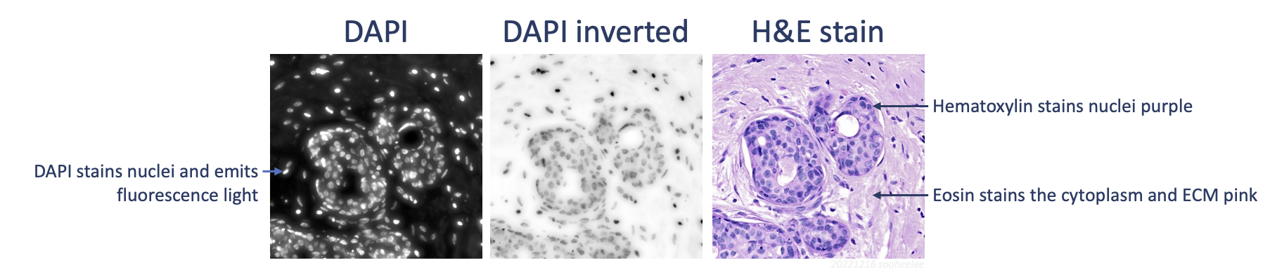
One necessary transformation for linear registration with automatic feature extraction is inversion of DAPI signal values. Given brightfield hematoxylin stains nuclei darkly and fluorescence DAPI illuminates nuclei brightly, the signals are negatively correlated. As such, we need to invert the DAPI signal, which is the first step in the next section. Should this approach give subpar registration results, consider adding a color deconvolution step (Image > Color > Colour Deconvolution 2 1,2 > H&E 2) to extract the hematoxylin stain to an 8-bit image from the H&E for better feature correspondence. For the tutorial’s example data, registration of the H&E to the inverted DAPI image gives usable results.
For researchers with plenty of RAM memory, BigWarp (Plugins>BigDataViewer>Big Warp) is a manual, interactive, landmark-based deformable (non-rigid) image alignment alternative. The manual landmark-based registration does not require image inversion or adjustment nor stacking the images.
Open the Series 3 DAPI morphology_mip-3.ome.tif image, which is 16-bit and 8854 x 6444 pixels, as well as the H&E stain morphology_he-shlee.png, which is RGB and 7519 x 5473 pixels. For visualization purposes, the DAPI image’s brightness and contrast were previously adjusted with Image > Adjust > Brightness/Contrast > Auto and then inverted as shown in step 3.1. The H&E image was previously sized and cropped.
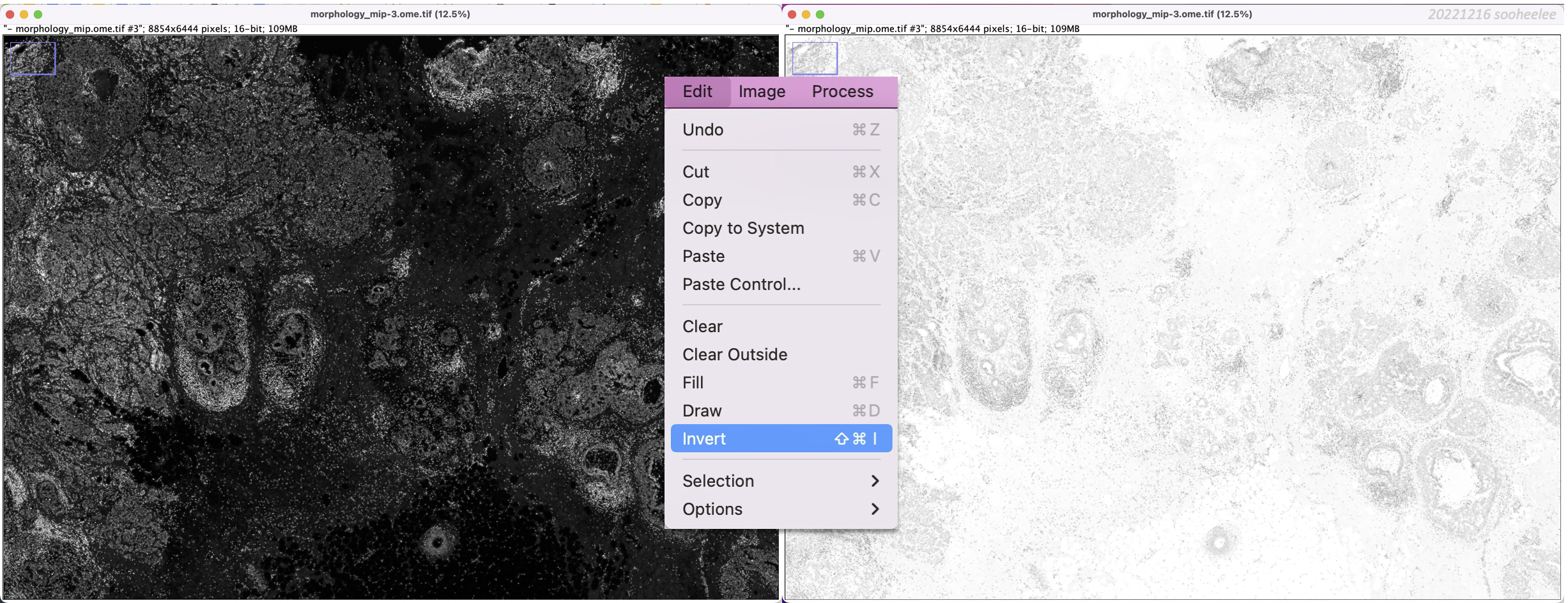
Step 3.1 Invert the DAPI signal
With the DAPI image window selected, go to Edit > Invert. This transforms the dark-background-image into a light-background-image, where the DAPI signal is dark.
Step 3.2 Create a stack of the DAPI and H&E images
Go to Image > Stacks > Images to Stack, then change the method to Scale (smallest).
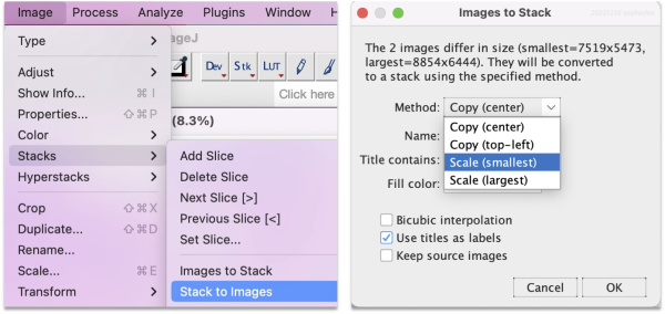
Choose the scaling option suitable for downstream analysis.
| What the option does | What step 3.3 results look like with the example data |
|---|---|
| Copy (center) recapitulates the smaller image, here the H&E, centered within the larger DAPI image dimensions. | Match the larger DAPI image dimensions, which enables use of Xenium scale factors to overlay cells or transcripts. Gives 219 features and the affine transform matrix [[1.174594988982544, -0.005845132439149, -743.5880948530574], [0.006058801885698, 1.173113560255031, -565.1019858709856]]. |
| Copy (top-left) recapitulates the smaller image, here the H&E, in the top-left corner of the larger DAPI image dimensions. | Match the larger DAPI image dimensions. Gives 236 features and the affine transform matrix [[1.174421395416202, -0.005700350622996, 36.77325277504045], [0.005803666083222, 1.17320514231513, 8.723536520371908]]. |
| Scale (smallest) reduces the larger image, the DAPI image, to match the scale of the smaller image, the H&E image. | Match the smaller H&E image dimensions. The tutorial uses this option as the H&E pixel size is already sized to 1 µm. Gives 304 features and the affine transform matrix [[0.997522382498024, -0.004711640834658, 30.872128429073182], [0.005300768713785, 0.996895147025494, 5.254392080997604]] |
| Scale (largest) increases the smaller image’s dimensions to match the larger image. For the example data, this setting alters the H&E image. | Match the later DAPI image dimensions. Gives 285 features and the affine transform matrix [[0.997332696231948, -0.005059889276386, 36.94356568847775], [0.004411193717504, 0.995787162740273, 10.94372313400254]]. |
The resulting two-layer image stack is in RGB and 7519 x 5473 pixels. Fiji supports the image type conversions shown at https://imagej.net/ij/docs/guide/146-28.html. While 16-bit to RGB conversion is possible, RGB color to grayscale is not.
Step 3.3 Register stack images with SIFT
Go to Plugins > Registration > Linear Stack Alignment with SIFT. Change the expected transformation to Affine and click OK. Wait a moment for the algorithm to run.
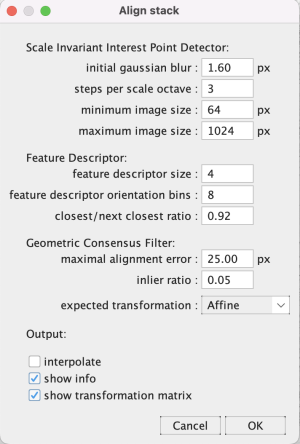
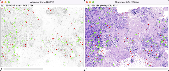
The optional alignment info windows (Output: show info) show non-matching and matching landmarks in different colors on a downsampled image stack. Checking the Output: show transformation matrix has the log print the affine transformation matrix*.
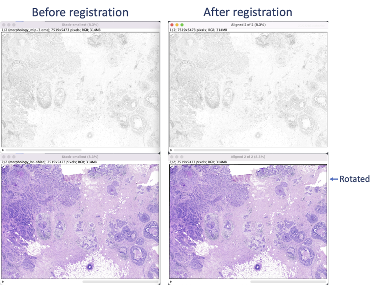
The registration results show a rotation in the H&E layer. The DAPI layer is unchanged. Toggling between the layers in a zoomed-in view shows offsets better (see GIFs at top). Press the triangular button in the lower-left of the window to have Fiji play through the layers on repeat.
For the example data, the relative coordinates in the registered H&E image match both Xenium cell and transcript XY coordinates. Save the aligned stack or convert it into individual images (Image > Stacks > Stack to Images) to save each image separately. Section [5] uses the single layer images.
Visually inspect the registration results using a Z projection and by overlaying Xenium transcripts or cell centroids onto the registered image.
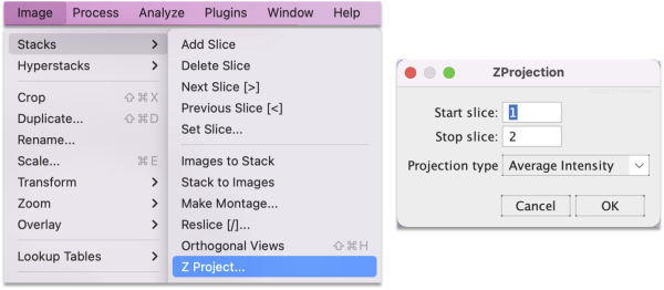
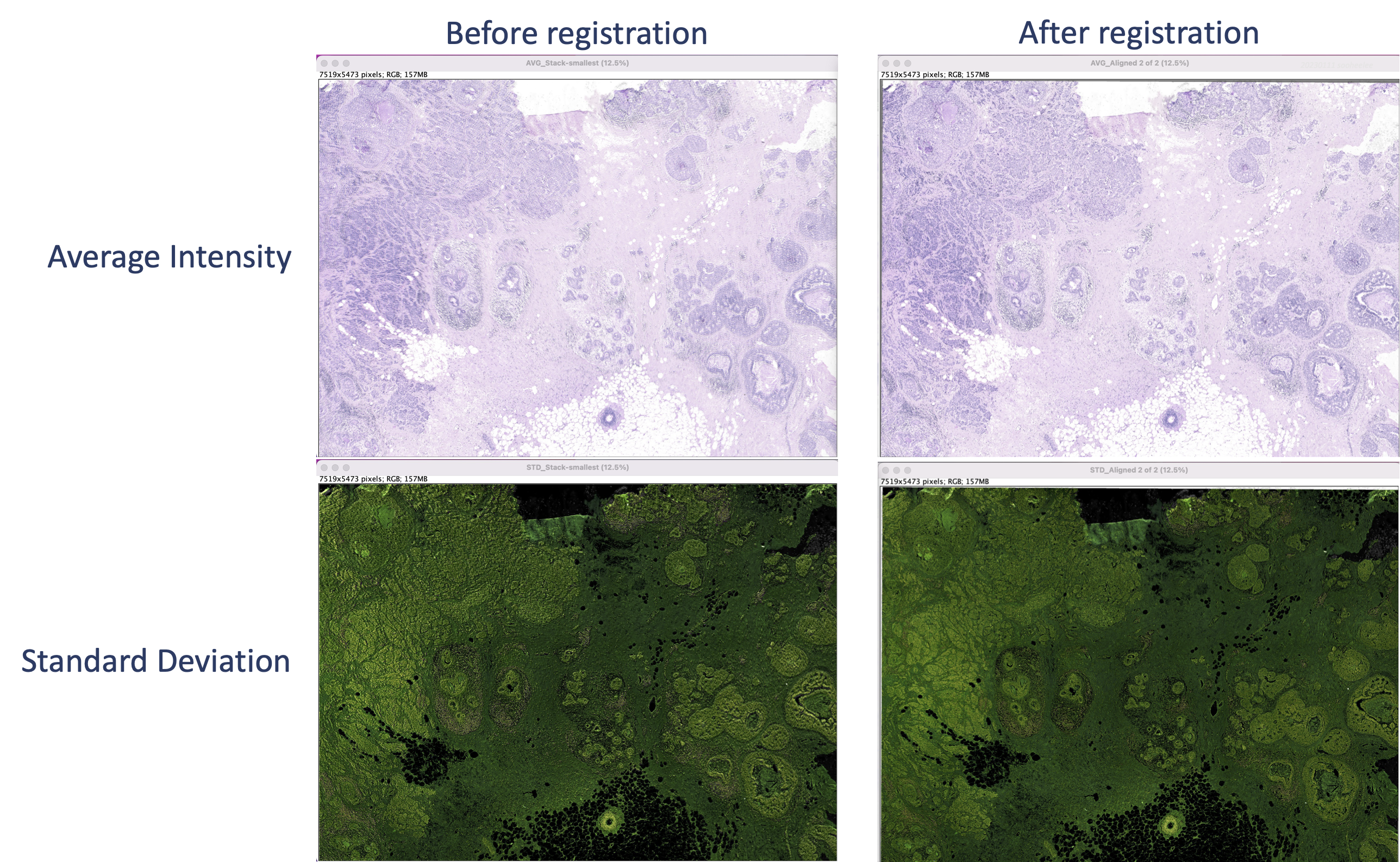
Step 4.1 Z project the stack layers
The Z projection creates a static image that highlights offsets. Perform steps on the original and the aligned stacks. Go to Image > Stacks > Z Project and for the projection type choose either Average Intensity or Standard Deviation.
This creates a merged image of the stack layers colorized by projection type. The average (top) shows a blurry starting image set and sharp features for the registered image set. For the standard deviation (bottom), the starting image set’s features appear shadowed or contoured, whereas the registered image set’s features are flat.
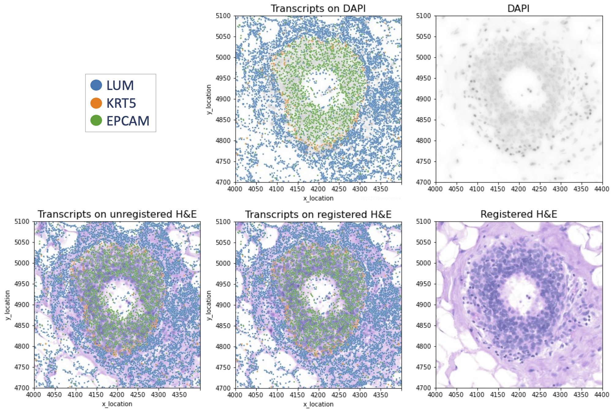
Step 4.2 Plot transcripts over H&E image using Python3
We overlay Xenium transcripts on the registered H&E image as well as on the DAPI image for comparison. Example DAPI-overlay code is here.
import pandas as pd
import seaborn as sns
import tifffile
from matplotlib import pyplot as plt
registered_he_url = ‘Aligned-0002.tif’
transcripts_url = 'outs/transcripts.parquet'
transcripts = pd.read_parquet(transcripts_url)
transcripts['feature_name'] = transcripts['feature_name'].apply(lambda x: x.decode('utf-8'))
# Subset transcripts to region of interest and quality value >= 20
subset = transcripts[
(transcripts['x_location'] > 4000) & (transcripts['x_location'] < 4400) &
(transcripts['y_location'] > 4700) & (transcripts['y_location'] < 5100) &
(transcripts['qv'] >= 20)]
# Define transcript features of interest
genes = ['LUM', 'KRT5', 'EPCAM']
# Plot registered H&E image
with tifffile.TiffFile(registered_he_url) as tif:
image = tif.series[0].levels[0].asarray()
plt.imshow(image, alpha=0.6)
# Plot transcripts
sns.scatterplot(
x = 'x_location', y = 'y_location',
data = subset[subset['feature_name'].isin(genes)],
hue = 'feature_name', s = 5, alpha = 1)
plt.title('Transcripts on registered H&E', size=16)
plt.legend(bbox_to_anchor=(1, 1), loc='upper left', ncol=1)
plt.axis('scaled')
plt.xlim(4000,4400)
plt.ylim(4700,5100)
plt.show()
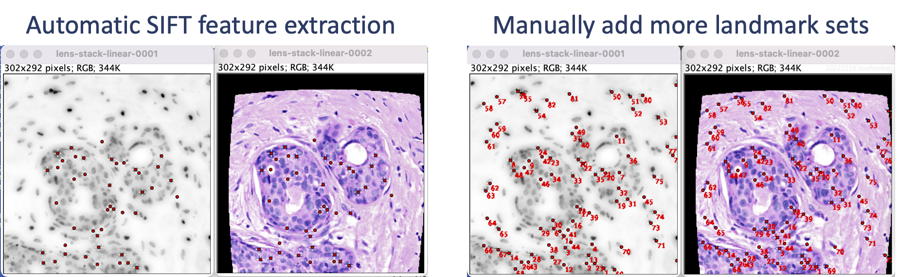
Keypoints mark corresponding features across images. We can use them with Fiji plugins, e.g. bUnwarpJ or BigWarp, or export them for use with custom coding solutions, e.g. apply a homography matrix from Fiji* to transform cell or transcript coordinates to then overlay on an unaltered image. Fiji enables automatic feature extraction with SIFT or MOPS algorithms as well as manual landmark selection interactively on the images. To illustrate, we use the registered tissue DAPI and H&E images from section [2]. Both images are RGB and 7519 x 5473 pixels.
Step 5.1 Extract features using SIFT or MOPS
Go to Plugins > Feature Extraction and choose either Extract SIFT Correspondences or Extract MOPS Correspondences. In the panel, set the expected transformation to Affine and press OK.
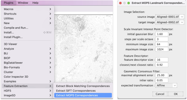
The algorithm takes a few seconds to extract and filter features. The SIFT and MOPS logs will show metrics on number of corresponding features and displacement.
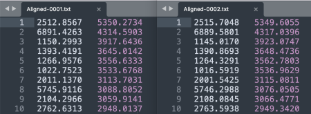
Step 5.2 Save the XY coordinates of extracted features
- As separate tables. For each image, save the XY coordinates of the keypoints with File > Save As > XY Coordinates. Each row tab-separates a keypoint's X and Y coordinates.
- In a single table. Alternatively, to save the keypoint sets in a single table, go to Plugins > Registration > bUnwarpJ. In the panel menu, choose the source versus target image, e.g. 0001 as the source and 0002 as the target. Click on the paper icon in the horizontal menu and then select Save Landarks As from the panel list that appears.
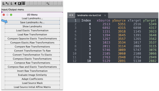
This saves the keypoint sets as a five-column table with pixel values rounded up to integers. The table lists an index, the source image X and Y coordinates, and then the target image X and Y coordinates.
Step 5.3 Manually add or modify keypoints
- With the bUnwarpJ module. bUnwarpJ can use landmarks extracted by Plugins > Feature Extraction and also allows for manual landmark manipulations from the module-specific horizontal menu. Details are in the Landmarks section of https://imagej.net/plugins/bunwarpj/.

The first button with the nib and plus sign allows adding keypoints. Adding a keypoint to one image causes a keypoint to appear in the second image in the same coordinate location, which is convenient. The second icon allows moving existing keypoints for more refined placement.
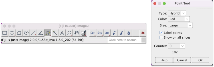
- With Fiji's multi-point tool, which is the seventh button in Fiji's floating menu showing five cross-hairs. Press the button with a single click, then click on the image to add a landmark. Double-click the button to bring up the Point Tool panel, which allows modifying how landmarks display, e.g. their size and color.
Non-rigid registration approach such as bUnwarpJ (Plugins > Registration > bUnwarpJ) or BigWarp (Plugins > BigDataViewer > Big Warp) may help address unusual registration needs, e.g. registering adjacent tissue slice images. We provide some discussion first on how these approaches are unsuitable for correcting flawed image preprocessing.
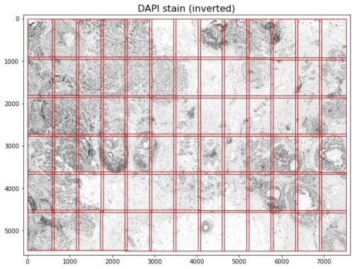
Microscope systems, including Xenium, capture images per field of view (FOV; as shown in red above for the v1.0 FOV demarcation). Software stitches together FOVs to create full-size images and typically automate image acquisition and stitching. In addition, imaging systems and software correct for the optical effects specific to each microscope's optics, e.g. barrel distortion or pincushion distortion, using compensating optics and software. If pipelines are improperly configured, images can manifest optical warping and stitching artifacts. The Xenium onboard analysis software corrects for per-FOV optical effects and performs FOV stitching to produce the full-size tissue image.
- The 12 x 24 mm full Xenium slide area produces approximately 33 x 19 (row x column) FOVs. Each FOV is 3520 x 2960 (row x column) pixels, and has 128-pixel overlaps with adjacent FOVs.
Ideally, image acquisition for different channels uses the same optics and algorithms for maximal correspondence of features across the stack layers. For two different microscopes, the same FOV boundaries and processing algorithms would enable the best correspondence. Realistically, two different microscope systems will use different FOV boundaries and different preprocessing. In such cases, in lieu of addressing a root distortion or artifact, registration per FOV, e.g. per-H&E-FOV registration to the Xenium DAPI image, may yield the best results. The optical distortion and stitching artifacts should present consistently across FOVs, given lenses and software are predictable. This enables deriving fine-resolution transformation models from feature-rich FOVs that can be applied across FOVs.
Correcting for lens distortion requires nonlinear transformation and is a fundamentally different problem from image registration. Fiji has a module to correct for lens distortion, e.g. Plugins > Transform > Distortion Correction, but we do not cover it here. Instead, we illustrate use of the elastic registration module bUnwarpJ with a small barrel-distorted H&E image and matching small DAPI image.
Step 6.1 Preprocess subset images
Perform linear registration with SIFT (section 3) and then feature extraction with SIFT (section 5). The result shows landmarks for nuclei-dense regions in the middle of the image. Manually add landmarks, e.g. using Fiji's multi-point tool (section 5.3) so the edges where the distortion is more pronounced have coverage.
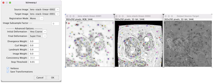
Step 6.2 Run bUnwarpJ on preprocessed images
Go to Plugins > Registration > bUnwarpJ. This brings up a panel menu.
- The algorithm transforms the source image (H&E) to register to the target image (DAPI).
- Change Registration Mode to Mono for unidirectional registration.
- In the advanced options change Landmark Weight from the default 0.0 to 0.9 so the algorithm heavily factors for the landmarks. Researchers should tune parameters appropriately for their data.
- Check Save Transformations to have the option to save the transformation coefficients.
After adjusting the parameters, click OK to run. The windows show activity.
When finished, a menu appears to save the transformation XY coefficients as a text file. After saving, a new window appears with the registration result.
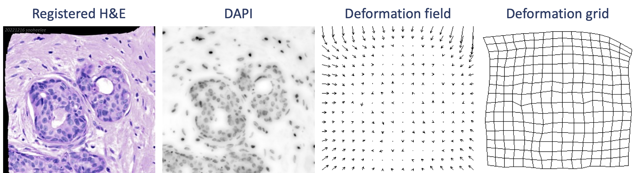
In the stack, the deformation field layer shows transformation vectors pointed inward in a pattern reminiscent of the shape of a lens. The top and left sides show larger vectors while the bottom and right sides show smaller vectors, where the registration looks better. Features at the very edge of the barrel on the right likely contributed to the better registration compared to the top and left. The deformation grid layer shows additional warping that is not symmetrical, which is unexpected from the symmetrical barrel distortion. This registration has room for improvement. The deformation grid suggests carefully placed all-manual landmarks may perform better.
Footnotes:
^ For ease of use with Fiji with 17 GB memory allocated.
* To convert a 3x2 affine transform matrix to a 3x3 homography matrix, simply append [0,0,1]. Packages for homography matrix transformation enable affine matrix transformations, e.g. OpenCV (cv2). See https://docs.opencv.org/4.x/d6/d00/tutorial_py_root.html and https://pypi.org/project/opencv-python/.