Goal: To evaluate the expression profiles of known gene markers of interest in the context of tissue morphology.
This tutorial will showcase how to obtain the spatial expression patterns of known gene markers associated with distinct cell types using a preloaded mouse brain dataset in Loupe Browser.
- Download and install Loupe Browser on either macOS or Windows.
- Familiarity with Loupe Browser navigation. Learn more in the Navigation Tutorial.
- Access the tutorial dataset.
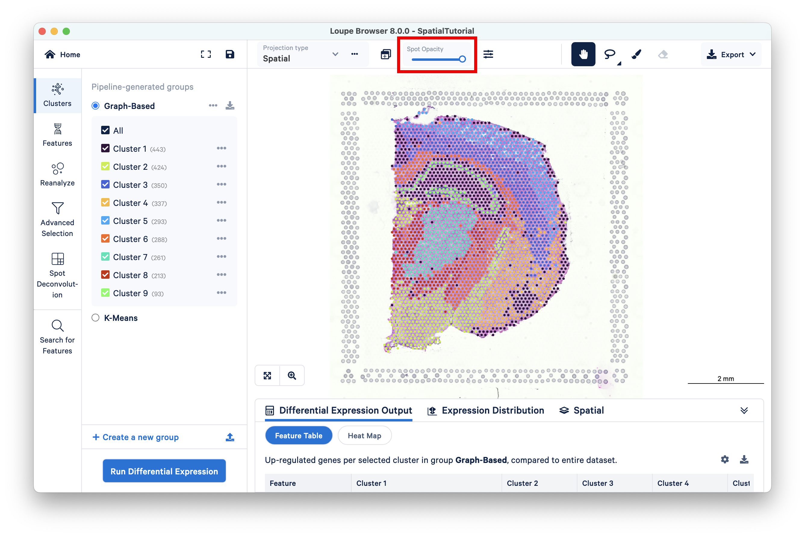
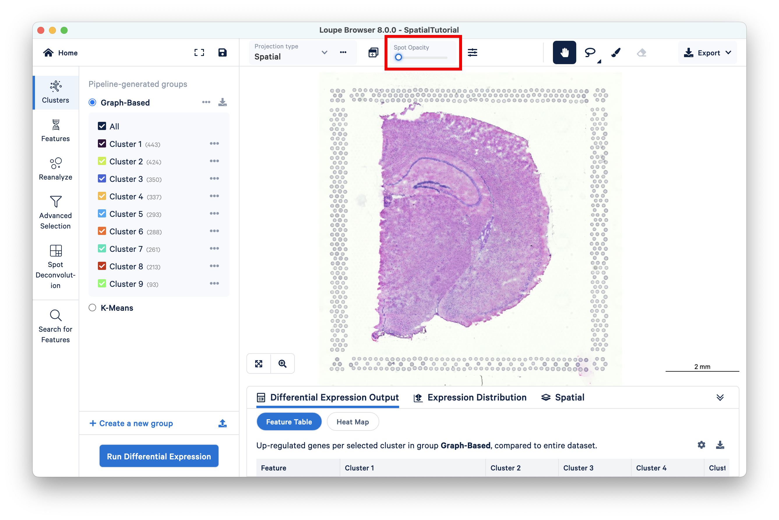
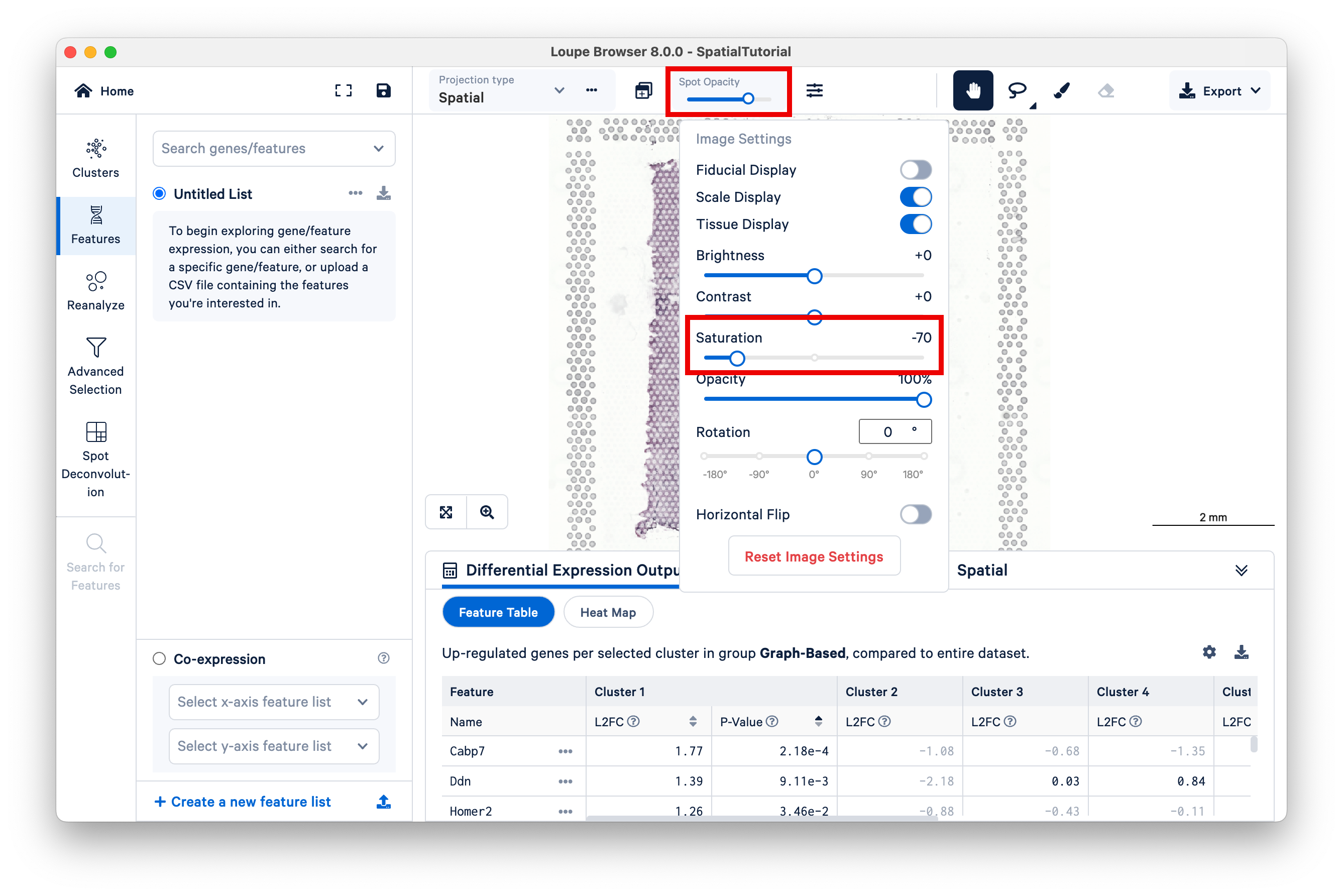
To evaluate gene expression data in the context of the H&E image, it is helpful to understand the underlying morphology. This can be achieved by making the spots transparent using the Spot Opacity slider:
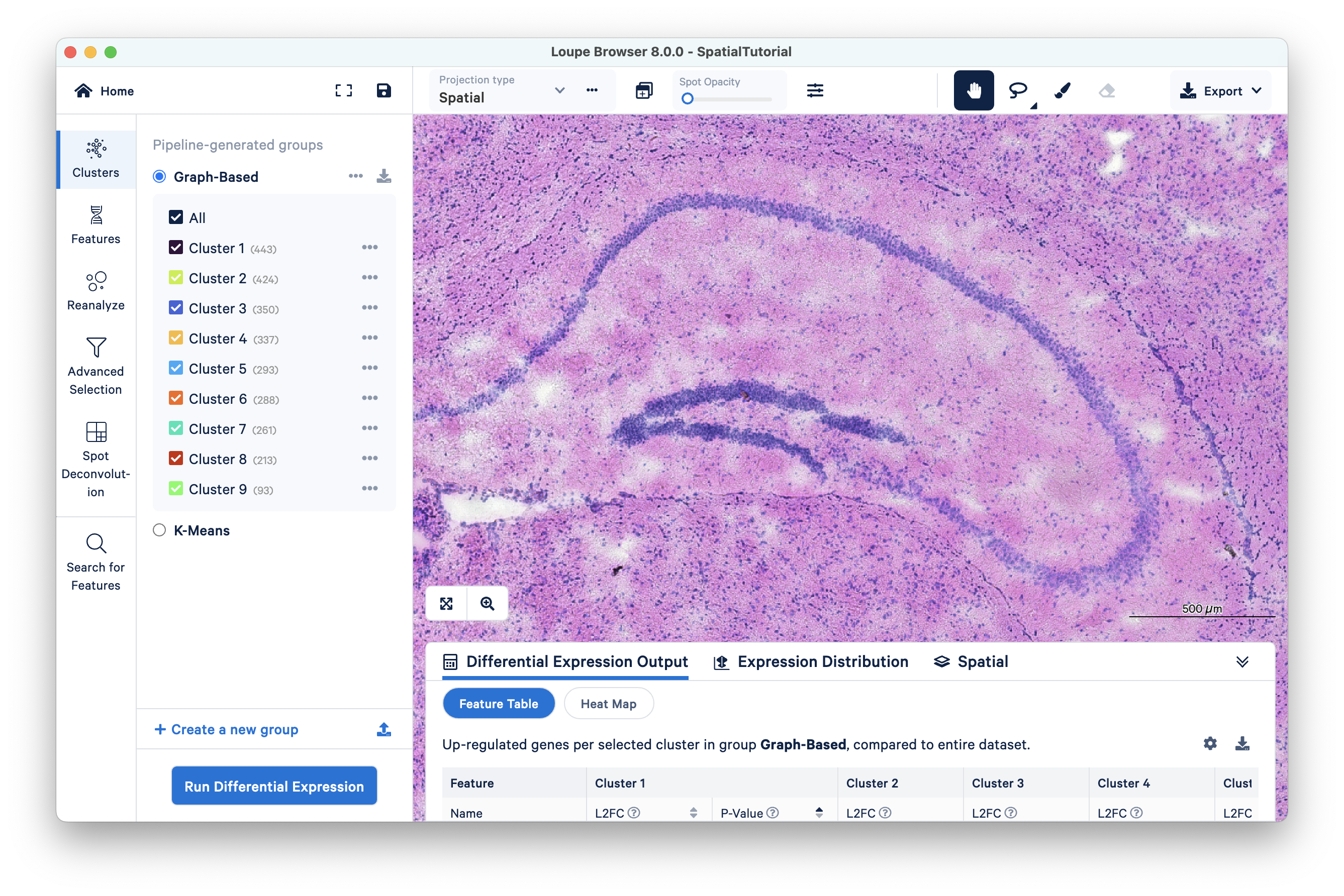
Using a combination of zoom and mouse dragging functionality navigate the image, evaluate the morphology, and identify landmarks of interest. You can zoom using either the mouse or the zoom slider. For example, in this image, the curvature of the hippocampus is highlighted in blue staining.
To autoscale back to default view, click ![]() .
.
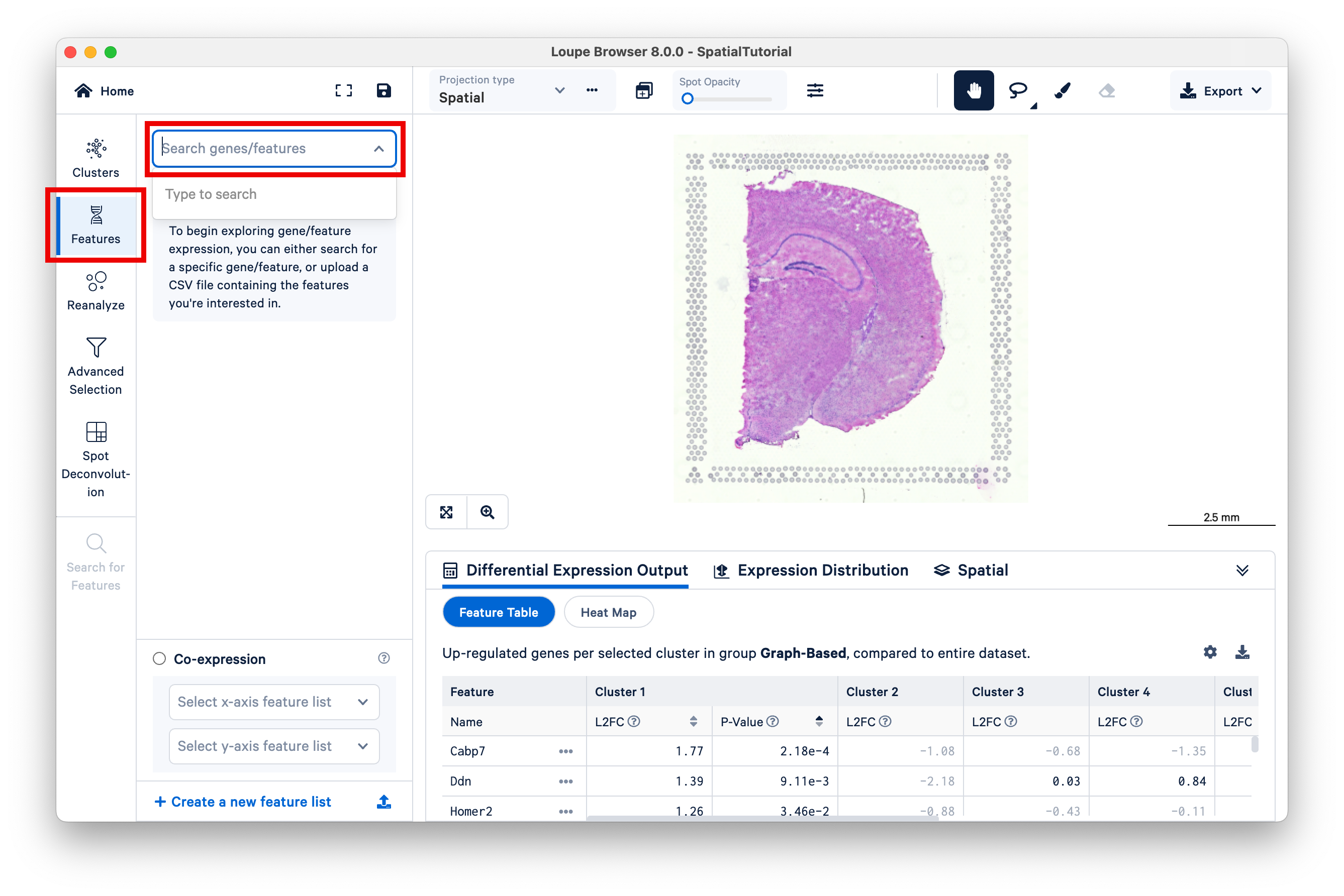
Loupe Browser can filter the expression for a specific gene, or list of genes. Click on Features, then Search genes/features to start typing.
To make the gene expression easier to visualize, make the spots opaque using the Spot Opacity slider, and reduce the saturation of the H&E image.
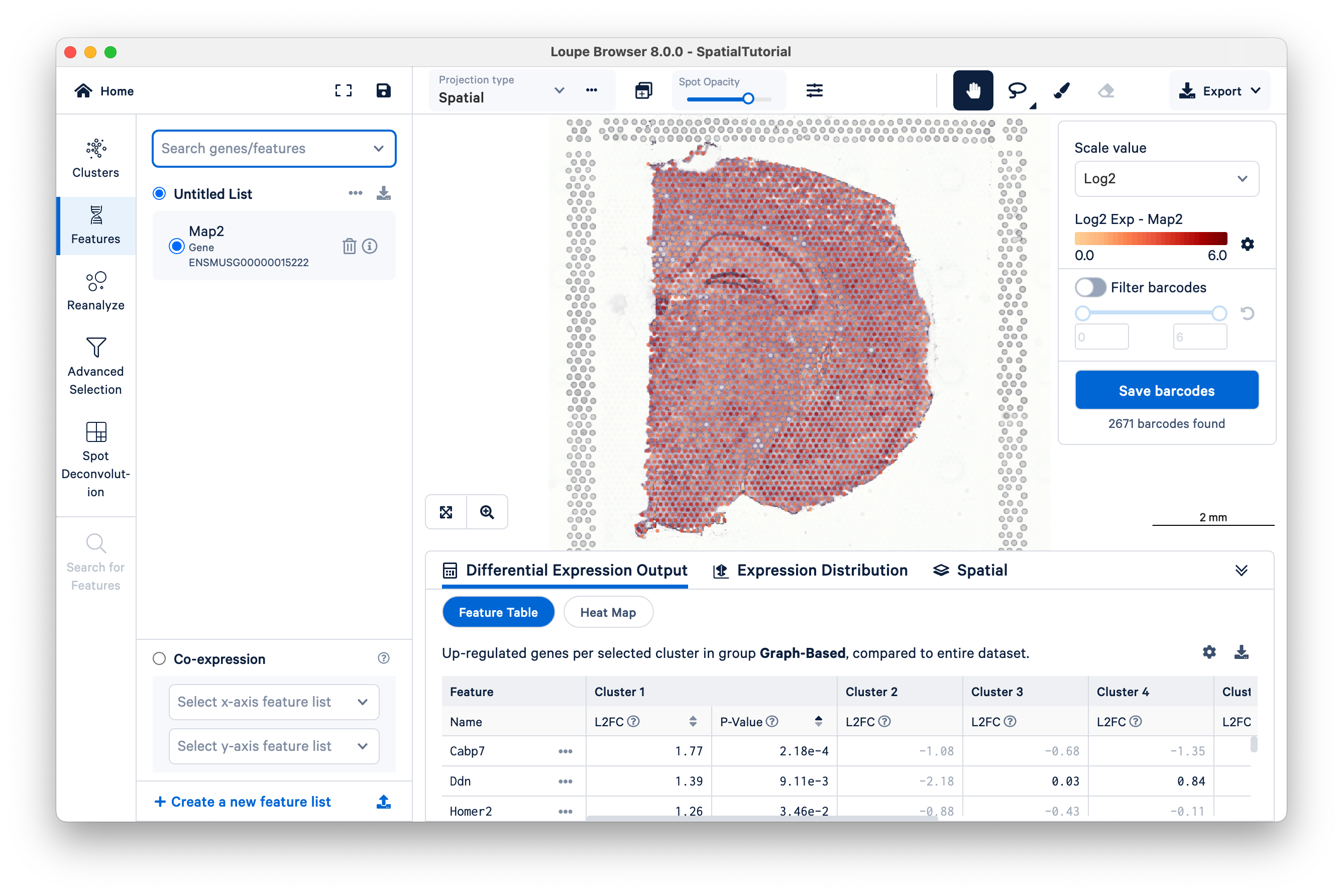
Next, we will explore the neuronal cell types using some well known markers. Search for Map2, which is responsible for microtubule protein that provides the structural support to neurons. The tissue image is then updated to color-coded spots based on the expression level of Map2 within that spot. As expected from general mature neuronal marker, high Map2 expression is spread across the tissue.
Click ![]() to load the Ensembl reference page for that gene as a new tab in web browser. Click
to load the Ensembl reference page for that gene as a new tab in web browser. Click ![]() to remove that gene from the current list.
to remove that gene from the current list.
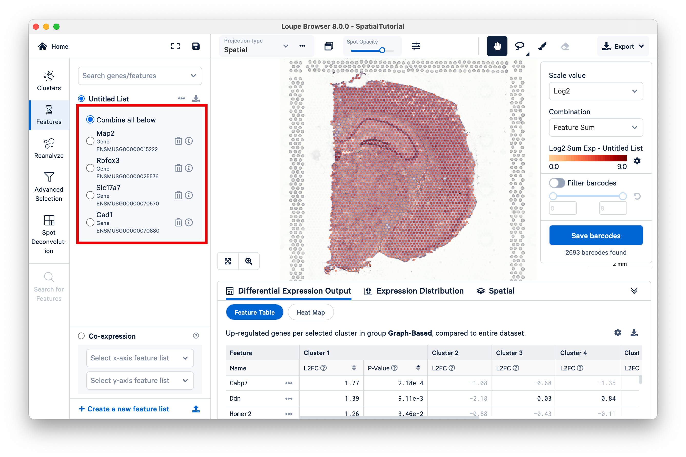
Next continue with these additional neuronal markers:
- Rbfox3, which is known to be important for neurogenesis and synaptogenesis, especially in the subgranular layer of the hippocampus
- Slc17a7 encodes a vesicle-bound, sodium-dependent transporter specifically found in glutamatergic neurons
- Gad1 encodes glutamic acid decarboxylase 67 which is crucial for gamma-aminobutyric acid (GABA) neurotransmission in neurons
These markers give a clear indication of the distinction in spatial expression. Rbfox3 and Slc17a7 are prominently expressed in excitatory neurons of the hippocampus and cerebral cortex, while Gad1 has a heavier presence in the inhibitory neurons of the thalamus. Click Combine all below. The resulting color signature represents a combination of expression levels across all the genes in the list. This allows you to visualize a set of genes associated with a cell type more confidently.
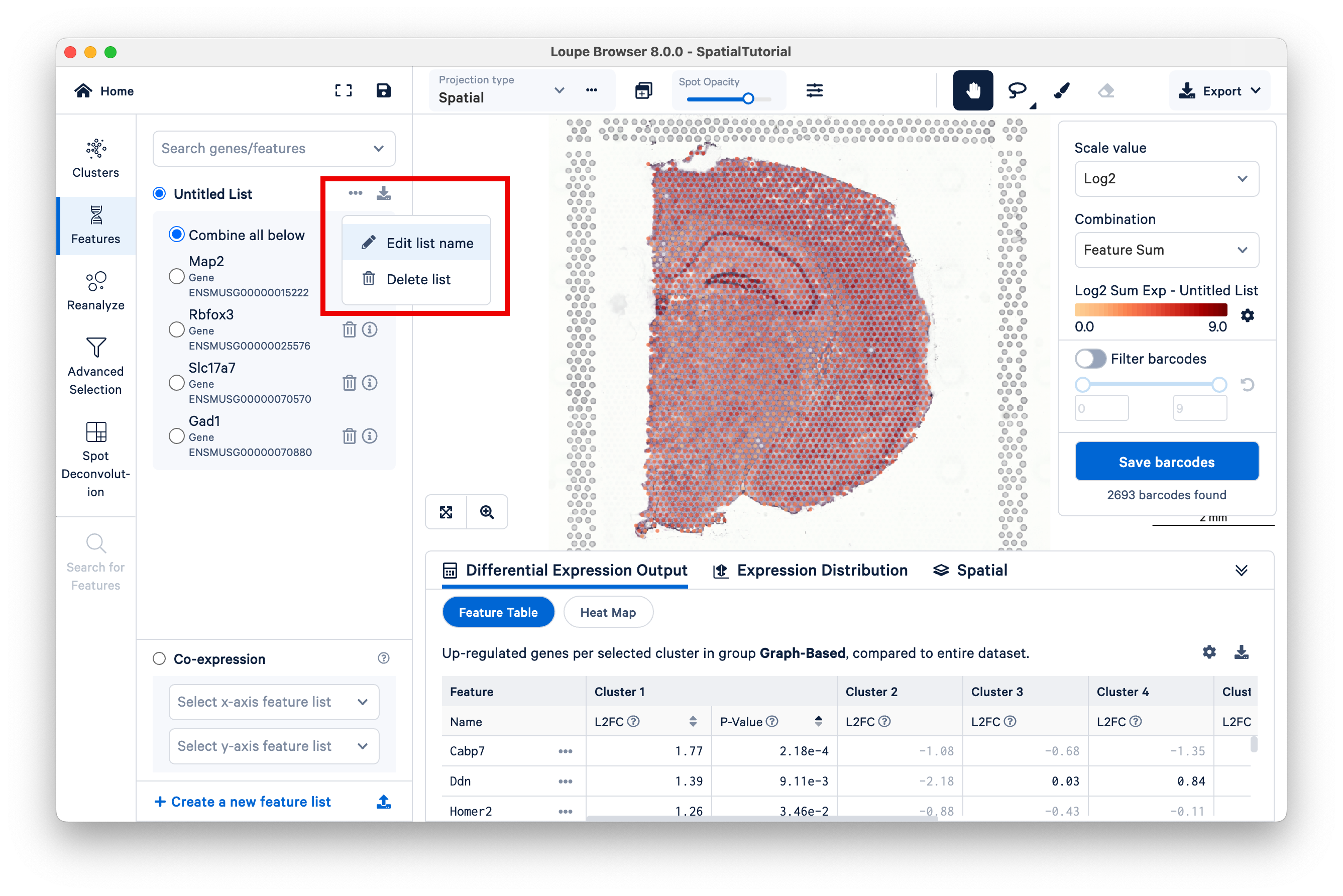
To finish, rename the Untitled List to Neuronal Markers.
Oligodendrocytes produce myelin sheaths that surround the axons of neurons. First, create a new feature list.

We will use two markers to identify this cell type:
- Mbp, which encodes the myelin basic protein, a major constituent of the myelin sheath
- Mog, which is a glycoprotein uniquely expressed on the surface of oligodendrocytes
As expected, strong expression of these markers coincides with anatomical locations of the major white matter tracks, including the corpus callosum, fimbria, cerebral peduncle, and optic track.

However, not all genes show definite patterns in spatial expression. As an example, look at some markers for microglia cells which are the resident immune cells:
- Cx3cr1 is a chemokine receptor highly expressed in microglia
- Tmem119 which is a cell-surface protein recently characterized as a microglial marker
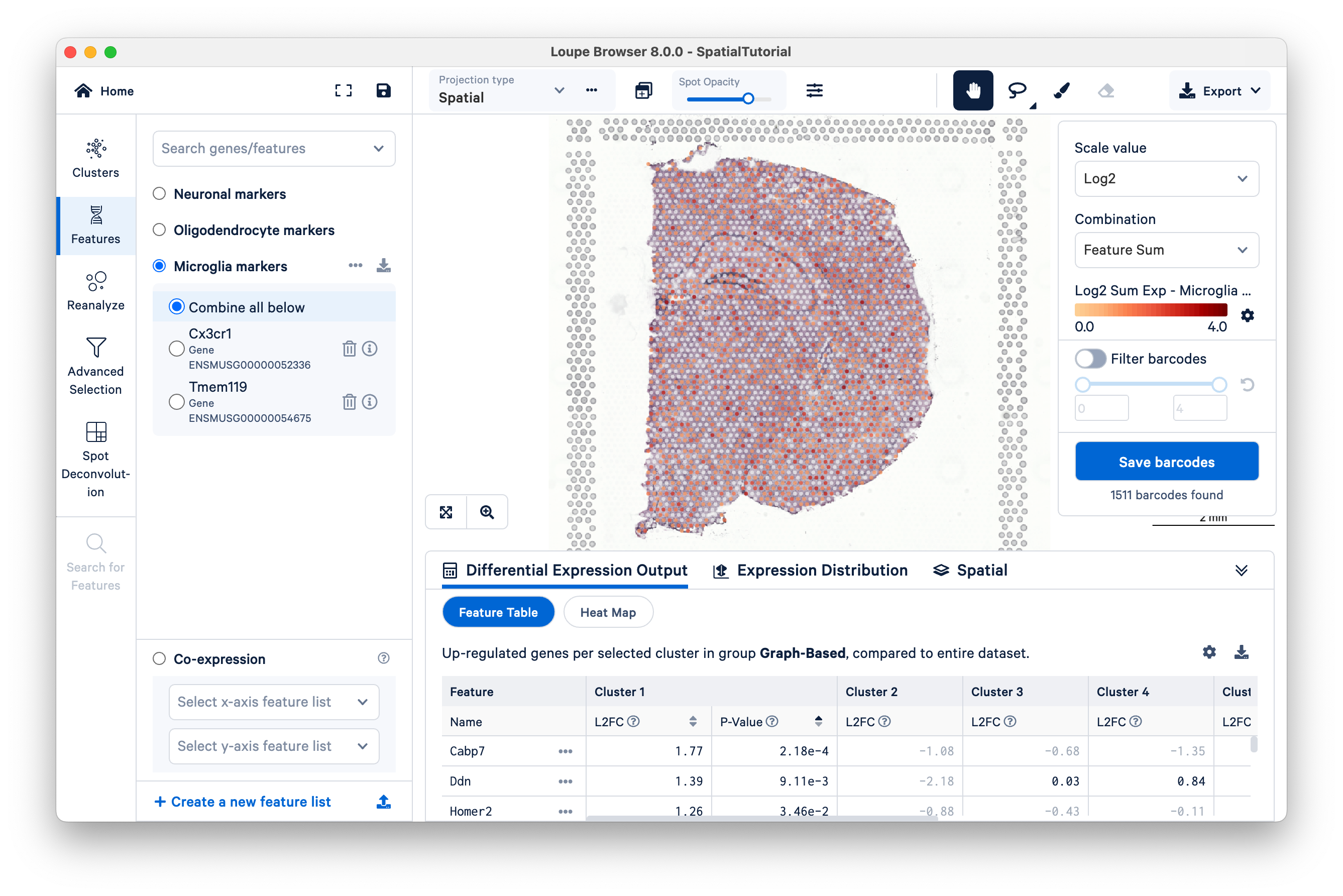
You can export the list as a CSV file:

The option to import a feature list is discussed in the Explore Spatial Clusters tutorial.
Another metric that is available to examine the spatial distribution of genes is by using the spatial correlation coefficient Moran's I which ranges from -1 (perfectly dispersed) to 1 (perfectly enriched). This metric is available for datasets analyzed using Space Ranger v1.3 or later.
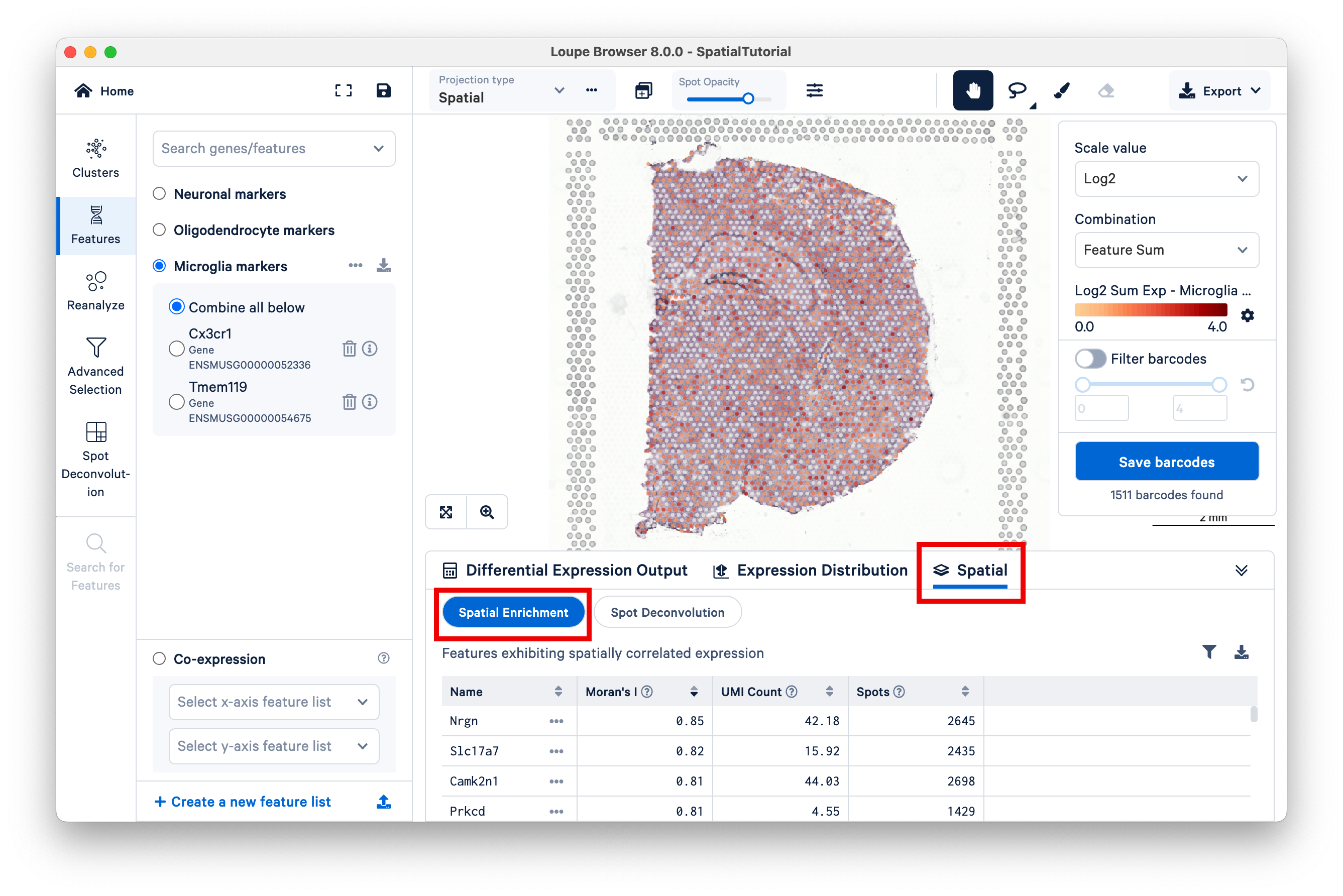
Click on Spatial, then Spatial Enrichment to access the spatial enrichment table. The features displayed in this table are filtered by Moran's I ≥0.05 and p-value ≤0.05 (p-value adjustment is performed using the Benjamini-Hochberg Procedure) and rounded to two decimal places to highlight the most spatially correlated features. The full list of Moran's I values for any dataset is captured in spatial_enrichment.csv which is generated in the outs/ folder after spaceranger count run.
The Spatial Enrichment table can be sorted by Moran's I value, UMI count, and the number of Spots for which at least one valid UMI is detected for the feature. The list of features can also be filtered by a specific Moran's I value range. The filtered and sorted list can be exported in CSV format. Clicking on the feature name pops a window with the option to add to Active Feature List.
We will now examine two sets of genes for examples to understand spatiality. For the first set, we choose genes Ttr and Defb11.
Ttr is detected across many spots (2674) and the Moran's I value is 0.81. The spatial pattern looks spread out with high expression in the lateral and third ventricles. On the other hand Defb11 is detected in a smaller number of spots (61), has Moran's I of 0.52 and the spatial pattern is localized to only the lateral and third ventricles. This is consistent with both the gene function and cell type association.
Ttr or Transthyretin encodes a carrier protein for thyroxine and retinol in cerebrospinal fluid (CSF) and is highly expressed in choroid plexus epithelial cells. However, its RNA has been detected in the cortex, hippocampus, and thalamus. Defb11 or Defensin beta 11 encodes an antimicrobial peptide and is expressed in choroid plexus epithelial cells. Since it is involved in innate immunity, the baseline expression is low.
For the second example, we will look at oligodendrocyte genes Mbp, Mobp and Mog.
A decreasing trend of highly expressed spots is visible moving from left to right in the tissue image. The spatial enrichment values in the table confirm the visual observation.
| Name | Moran's I | UMI Count | Spots |
|---|---|---|---|
| Mbp | 0.8 | 112.88 | 2700 |
| Mobp | 0.74 | 28.47 | 2595 |
| Mog | 0.57 | 5.41 | 1984 |
This is consistent with cell type association. Mbp and Mobp are associated with myelin forming and mature oligodendrocytes. They are also expressed in excitatory, inhibitory, and cholinergic neurons in the hindbrain as well as afferent nuclei of cranial nerves. Mog, on the other hand, is only associated with myelin-forming and mature oligodendrocytes and hence shows lower spatial clustering.
Using the methods shown in the tutorial, you can map known gene markers to spots, overlay that information on top of the tissue image, and use that to verify that the expected gene patterns are present in their respective brain tissue types.
In the next section, we will explore spatial clusters.