Note: 10x Genomics does not provide support for community-developed tools and makes no guarantees regarding their function or performance. Please contact tool developers with any questions. If you have feedback about Analysis Guides, please email analysis-guides@10xgenomics.com.
Trajectory inference from single cell gene expression data can be used to reconstruct the dynamic processes that cells undergo as part of their true biological nature, including differentiation, maturation, response to stimuli, and cell cycle. To improve the inferred trajectories, RNA velocity methods leverage the information of unspliced and spliced transcripts levels to estimate the future state of a single cell (https://www.nature.com/articles/s41586-018-0414-6).
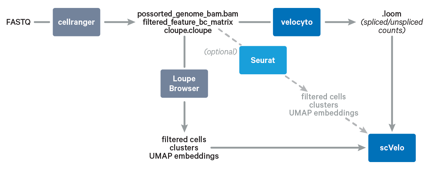
In this Analysis Guide Tutorial, we provide you with the instructions to import results obtained with Cell Ranger and Loupe Browser into community-developed tools for RNA velocity analysis. Below is an overview of the tools and main files involved in this Analysis Guide.
Required:
You will need to install the following software packages in order to run the analysis in this guide. For installation instructions, please refer to the websites for each of the tools.
Highly recommended:
- Access to a Linux server and being able to run the python packages on the server. This is because the
velocytopipeline requires large amounts of computing resources. - Jupyter Notebook is an interactive computing platform. Within the Jupyter Notebook, you can see both the code and the results, and run cell by cell to better understand the code.
Optional:
In this guide, we will use a neutrophil dataset as an example for trajectory analysis. You can download the raw FASTQ files from the link above and follow the tutorial Capturing Neutrophils in 10x Single Cell Gene Expression Data to obtain input files for this analysis guide.
We included key intermediate files and expected outputs for your reference. If you are only interested in running scVelo, you can use the files we provided. However, if you want to start from raw data or velocyto step, you will need to run Cell Ranger according to the neutrophil tutorial.
If you would like to use your own Single Cell Gene Expression data to run the velocity analysis in this guide, you need the output directory from Cell Ranger (including the outs/ subdirectory).
Step 1. Export projection and clusters from Loupe Browser
The dataset we are using contains neutrophils and other blood cells, but here we are only interested in performing trajectory analysis on neutrophils. Therefore, the first step is to annotate the cell types and export relevant information (projections and clusters) for only neutrophils.
Steps for raw data process and cell type annotation are detailed in Tutorial: Capturing Neutrophils in 10x Single Cell Gene Expression Data. After following the steps in the above tutorial, we need to export the neutrophil-only UMAP embeddings and clusters from the neutrophil reclustering results. Details of how to export projects and clusters can be found here.
For your reference, the files are provided here for download.
Step 2. Prepare conda environment
We recommend using conda for the following parts of the tutorial. Please follow the installation instructions for your preferred operating system.
We have prepared a yaml file to facilitate the installation of the necessary packages to run each of the steps in this tutorial. This yaml file contains a list of library packages that the conda manger will use to install the necessary libraries for you to import later. Please download this yaml file and make sure it is located in the same directory where you will execute the following conda command. Once conda is installed, run the following command to create the environment.
conda env create --file TutorialEnvironment.yml
Tip: You can change the first line of the yaml file to change the name of the environment. The current name is name: tutorial.
Step 3. Run velocyto
For velocity analysis, we will first use the velocyto pipeline (La Manno et al., Nature, 2018) to obtain the pre-mature (unspliced) and mature (spliced) transcript information based on Cell Ranger output.
We have already prepared the conda environment in the earlier step. To activate the environment for this and the next step in the guide, we can run this command:
conda activate tutorial
The velocyto pipeline requires two inputs:
- The Cell Ranger output directory, which contains the subfolders
outs,outs/analysis, etc. - A genome annotation (GTF file). This needs to be the same GTF in the reference used to run Cell Ranger. Tip: you can find the reference path in the Web Summary Sample section.
Once you have the paths to these two inputs, you can run velocyto with the following command (be sure to replace path/to with the actual file paths on your server).
velocyto run10x /path/to/cellranger-runs/sample_name /path/to/refdata-gex-GRCh38-2020-A/genes/genes.gtf
velocyto pipeline takes a long time to complete and requires high amounts of resources (include RAM/CPUs). We recommend running this part of the tutorial in a HPC cluster or a high-end workstation.When the pipeline completes successfully, the output velocyto/sample_name.loom will be in the Cell Ranger output directory specified as input in the command line. More information about the .loom file can be found in the velocyto User Guide.
In case you would like to jump to the next step of the tutorial, here is the output of the velocyto pipeline: loom file.
Step 4. Run scVelo
In this section, we use scVelo (Bergen et al., Nature Biotech, 2020) to recover and visualize RNA velocity. scVelo is a scalable toolkit that leverages splicing kinetics for RNA velocity analysis.
Here is a Jupyter notebook file that you can download to use for this tutorial. Click on the following button to interact with this Jupyter notebook file using Google Colab:
4.1 Download input files
scVelo requires files generated from the earlier steps. However, if you prefer skipping the earlier steps, you can download the input files needed by scVelo from here:
- Filtered feature-barcode matrix
.loomfile: spliced/unspliced counts fromvelocyto- Neutrophil Clusters exported from Loupe Browser
- Neutrophil UMAP exported from Loupe Browser
You could also use curl command to download the files to your server:
mkdir input-files
curl -o input-files/filtered_feature_bc_matrix.tar.gz https://cf.10xgenomics.com/supp/cell-exp/neutrophils/filtered_feature_bc_matrix.tar.gz
curl -o input-files/WB_Lysis_3p_Introns_8kCells.loom https://cf.10xgenomics.com/supp/cell-exp/neutrophils/WB_Lysis_3p_Introns_8kCells.loom
curl -o input-files/3p-Neutrophils-clusters.csv https://cf.10xgenomics.com/supp/cell-exp/neutrophils/3p-Neutrophils-clusters.csv
curl -o input-files/3p-Neutrophils-UMAP-Projection.csv https://cf.10xgenomics.com/supp/cell-exp/neutrophils/3p-Neutrophils-UMAP-Projection.csv
tar -xvzf input-files/filtered_feature_bc_matrix.tar.gz -C input-files/
ls -lahR input-files
The commands above will create a directory called input-files, download the files required for this tutorial section, and extract the files into this directory. In the steps below, we will refer to the Path of this directory for input files.
4.2 Open jupyter notebook and import libraries
We recommend following the steps below with Jupyter Notebook, where you can interactively explore the functions and data. You can run this in Google Colab, or with Jupyter notebook on your local computer.
If you are using your local computer, open a new Jupyter environment with the following command, then start a new Python notebook:
jupyter notebook
Once you start a new notebook, then you can copy-and-paste the code blocks below into your notebook to run the analysis. To start, import required packages in the current session:
import numpy as np
import pandas as pd
import matplotlib.pyplot as pl
import scanpy as sc
import igraph
import scvelo as scv
import loompy as lmp
import anndata
import warnings
warnings.filterwarnings('ignore')
Note: if you run the section above to import the packages and get a warning message, e.g. "ModuleNotFoundError: No module named 'loompy'" this means that these libraries were not installed. Please see "Step 2. Prepare conda environment" above for instructions on how to install these packages in an environment with this yml file. Or, as an alternative if you are unable to get conda to work, you can run this line to manually install the Python libraries using the latest version of the pip installer instead:
python -m pip install --upgrade pip
pip install numpy pandas matplotlib scanpy igraph scvelo loompy anndata
We can customize the plot colors and sizes by changing the visualization settings:
# Set parameters for plots, including size, color, etc.
scv.set_figure_params(style="scvelo")
pl.rcParams["figure.figsize"] = (10,10)
Colorss=["#E41A1C","#377EB8","#4DAF4A","#984EA3","#FF7F00","#FFFF33","#A65628","#F781BF"]
4.3 Import matrix
Next, import the filtered gene expression matrix output from Cell Ranger into scVelo.
# Define Path to the matrix output from cellranger
Path10x='./input-files/filtered_feature_bc_matrix/'
# Read matrix
Neutro3p = sc.read_10x_mtx(Path10x,var_names='gene_symbols',cache=True)
# Print information on this new object
Neutro3p
The output of Neutro3p should be:
AnnData object with n_obs × n_vars = 8000 × 36601
var: 'gene_ids', 'feature_types'
Tip: If you filtered your matrix using Seurat, you can load the .loom output from Seurat using this function: Neutro3p = scv.readloom("./Neutro3pSeurat.loom"). More detail is provided in the alternative steps section at the end of this guide.
4.4 Import clusters and projection
Next, import the clusters and UMAP embeddings from Loupe Browser (Step 1), so that we can use these information when making plots in scVelo.
# Read clusters
Clusters_Loupe = pd.read_csv("./input-files/3p-Neutrophils-clusters.csv", delimiter=',',index_col=0)
# Create a list with only neutrophil Barcodes, because the dataset included other cell types.
Neutrophils_BCs=Clusters_Loupe.index
# Read UMAP embeddings
UMAP_Loupe = pd.read_csv("./input-files/3p-Neutrophils-UMAP-Projection.csv", delimiter=',',index_col=0)
# Select neutrophil barcodes in the projection
UMAP_Loupe=UMAP_Loupe.loc[Neutrophils_BCs,]
# Tansform to Numpy
UMAP_Loupe = UMAP_Loupe.to_numpy()
# Filter cells for only neutrophils
Neutro3p=Neutro3p[Neutrophils_BCs]
# Import cluster information into Neutro3p object
Neutro3p.obs['Loupe']=Clusters_Loupe
# Import UMAP information into Neutro3p object
Neutro3p.obsm["X_umap"]=UMAP_Loupe
# Print information about the object
Neutro3p
The Neutro3p object now includes additional information:
AnnData object with n_obs × n_vars = 3343 × 36601
obs: 'Loupe'
var: 'gene_ids', 'feature_types'
obsm: 'X_umap'
4.5 Import spliced/unspliced counts
scVelo requires pre-mature (unspliced) and mature (spliced) transcript information, which was obtained in Step 3 with velocyto. Now, we will read in the velocyto output and merge these counts into the Neutro3p object.
# Read velocyto output
VelNeutro3p = scv.read('./input-files/WB_Lysis_3p_Introns_8kCells.loom', cache=True)
# Merge velocyto with cellranger matrix
Neutro3p = scv.utils.merge(Neutro3p, VelNeutro3p)
4.6 Run velocity analysis
With all of the required information loaded, we can process the dataset and obtain latent time values for each cell.
# Standard scvelo processing to run Dynamical Mode
scv.pp.filter_and_normalize(Neutro3p, min_shared_counts=30, n_top_genes=2000)
scv.pp.moments(Neutro3p, n_pcs=30, n_neighbors=30)
# Estimate RNA velocity and latent time
scv.tl.recover_dynamics(Neutro3p)
scv.tl.velocity(Neutro3p, mode='dynamical')
scv.tl.velocity_graph(Neutro3p)
scv.tl.recover_latent_time(Neutro3p)
4.7 Visualization
After the analysis, we can visualize the velocity results using different type of plots.
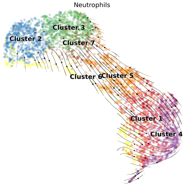
(1) We can visualize the velocities in UMAP embedding and color the cells by the cluster assignments exported from Loupe Browser:
# Generate plot with UMAP and cluster
scv.pl.velocity_embedding_stream(Neutro3p,basis="umap",color="Loupe",title='Neutrophils',fontsize=20,legend_fontsize=20,min_mass=2,palette=Colorss,save='scVelo-umap-cluster.png')
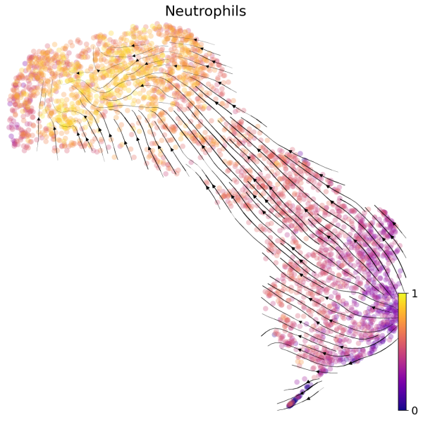
(2) We can also visualize the velocities in UMAP embedding with latent time. The latent time represents the cell’s internal clock and approximates the real time experienced by cells as they differentiate.
# Generate plot with UMAP and latent time
scv.pl.velocity_embedding_stream(Neutro3p,basis="umap",color="latent_time",title='Neutrophils',fontsize=20,legend_fontsize=20,min_mass=2,color_map="plasma",save='scVelo-umap-latent_time.png')
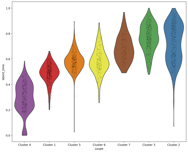
(3) We can visulize the latent time for each cluster using a violin plot. The result is consistent with what we observed in the two plots above.
sc.pl.violin(Neutro3p, keys='latent_time',groupby="Loupe",order=["Cluster 4","Cluster 1","Cluster 5","Cluster 6","Cluster 7","Cluster 3","Cluster 2"],save='scVelo-violin-latent_time.png')
(4) Since we are analyzing nuetrophils, we use a list of genes that are differentially expressed during neutrophil maturation (Combes et al. 2021). We plot the expression of these genes in each cell sorted with their latent time.
Genes=["RETN","LTF","CAMP","ACTB","GCA","LCN2",
"S100A8","MYL6","S100A9","FCGR3B","S100A11","FTH1","IFIT1",
"IFITM3","IFIT3","ISG15","IFIT2","RPS9","NEAT1","MALAT1","NFKBIA","CXCL8"]
scv.pl.heatmap(Neutro3p, var_names=Genes, sortby='latent_time', col_color='Loupe', n_convolve=100,figsize=(16,8),yticklabels=True,sort=True,colorbar=True,show=True,layer="count",save='scVelo-heatmap-latent_time.png')
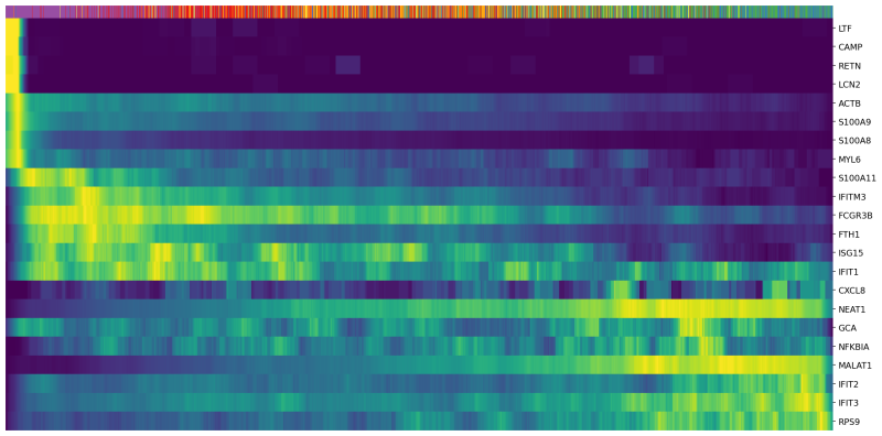
In the heatmap above, cells were ordered by latent time (the top bar, more recent on the right). Immature neutrophil marker genes, such as LTF and LCN2, have higher expression levels (yellow) in the cells with earlier latent time. This indicates that the transcriptional dynamics in our neutrophils are consistent with the observations in the previous publications.
If you have already done analysis in Seurat, you could also import your Seurat object into the trajectory analysis. In this section, we describe how to export a Seurat object from R, and then import it into Python for velocity analysis.
This section assumes R is already installed, and standard Seurat processing is completed. You can save the Seurat object as a .loom file using the function below in R:
## This step is done in R after Seurat processing
Neutro3p.loom <- as.loom(Neutro3p, filename = "/path/to/Neutro3pSeurat.loom", verbose = FALSE)
Neutro3p.loom$close_all()
This Seurat loom file can then be loaded into scVelo using scv.read_loom function (replacing the sc.read_10x_mtx), shown in Step 4.3 above.
In this analysis guide, we provide a step-by-step tutorial on how to perform velocity analysis on 10x Genomics Single Cell Gene Expression data. Although neutrophil are used here, the same analysis process can be applied to other cell types of your interest.
We used velocyto and scVelo in this guide. However, there are other community developed tools for trajectory inference and velocity analysis. For further reading, please see these reviews: