In this guide, we provide an overview of best practices for analyzing single cell gene expression data generated using the Chromium platform from 10x Genomics, along with an example experimental setup for multiple datasets. This guide outlines the standard steps for getting started with the analyses, with practical tips and recommendations to help achieve reliable results.

While we will cover the common steps of all single cell gene expression data analyses such as quality control, normalization, clustering, differential expression analysis, cell type annotation, and data integration, this article is not exhaustive and will not delve into more specialized analyses such as trajectory inference, integration of multimodal data, or cell-cell communication. This article will focus on gene expression data and will not cover other data modalities such V(D)J, antibody, CRISPR, or ATAC.

To demonstrate the analysis flow, we will use four datasets from the 10x Genomics support site:

• 5k Human PBMC (Donor 1), male, aged 18-35
• 5k Human PBMC (Donor 2), male, aged 18-35
• 5k Human PBMC (Donor 3), female, aged 36-50
• 5k Human PBMC (Donor 4), female, aged 36-50

These healthy human PBMC samples were generated using the Chromium GEM-X Single Cell 3' Reagent Kits v4. Each dataset comes from an individual GEM well. While these specific samples serve as a practical example, the biological story itself is not the primary focus. We will process these samples to identify sex-based differences in cell types, showcasing a complete analysis flow. The analysis steps presented are broadly applicable to diverse research questions, sample types, and experimental conditions, allowing adaptation for various single cell transcriptomic studies.

To follow the analysis flow discussed in this guide, ensure you have completed the following:

1. Create a 10x Genomics Cloud Analysis account: If you intend to utilize the 10x Genomics Cloud Analysis platform for processing or managing your data, setting up an account is required. You can sign up for an account here. See this page for instructions on account creation. Some regions may not have access to 10x Cloud Analysis (see here for detail), and installation of command line-based software tools may be required.
2. Loupe Browser software installation: For interactive visualization and exploration of 10x Genomics single cell data, download and install Loupe Browser. Download the software from this page and follow the instructions for installation.

The raw reads in FASTQ files can be processed using Cell Ranger. Cell Ranger is a set of analysis pipelines that process Chromium single cell data to align reads, generate feature-barcode matrices, and perform clustering and other secondary analyses. See What is Cell Ranger? for an overview of what Cell Ranger can do.

Cell Ranger can be run on the 10x Genomics Cloud or through the command line on your own computing infrastructure after download and installation. We recommend those who are getting started with their single cell analyses run Cell Ranger on the 10x Genomics Cloud because of its ease of use and fast processing times.

Set up the analysis on 10x Cloud

To process FASTQ files of the example GEM-X PBMC datasets, we will be using the Cell Ranger multi pipeline on the 10x Cloud, which performs read alignment, UMI counting, cell calling, clustering, and cell type annotation. Note that each analysis with the Cell Ranger multi pipeline only processes data from the same GEM well. For the four example datasets, we will analyze each of them individually at this stage, as they came from four individual GEM wells. The steps include:

1. Create a project in your Cloud Analysis account: Projects are where you upload data and run analysis pipelines. You can upload different samples to a single project.

2. Upload the FASTQ files via web browser or CLI. For the easiest functionality, we recommend using the web browser.

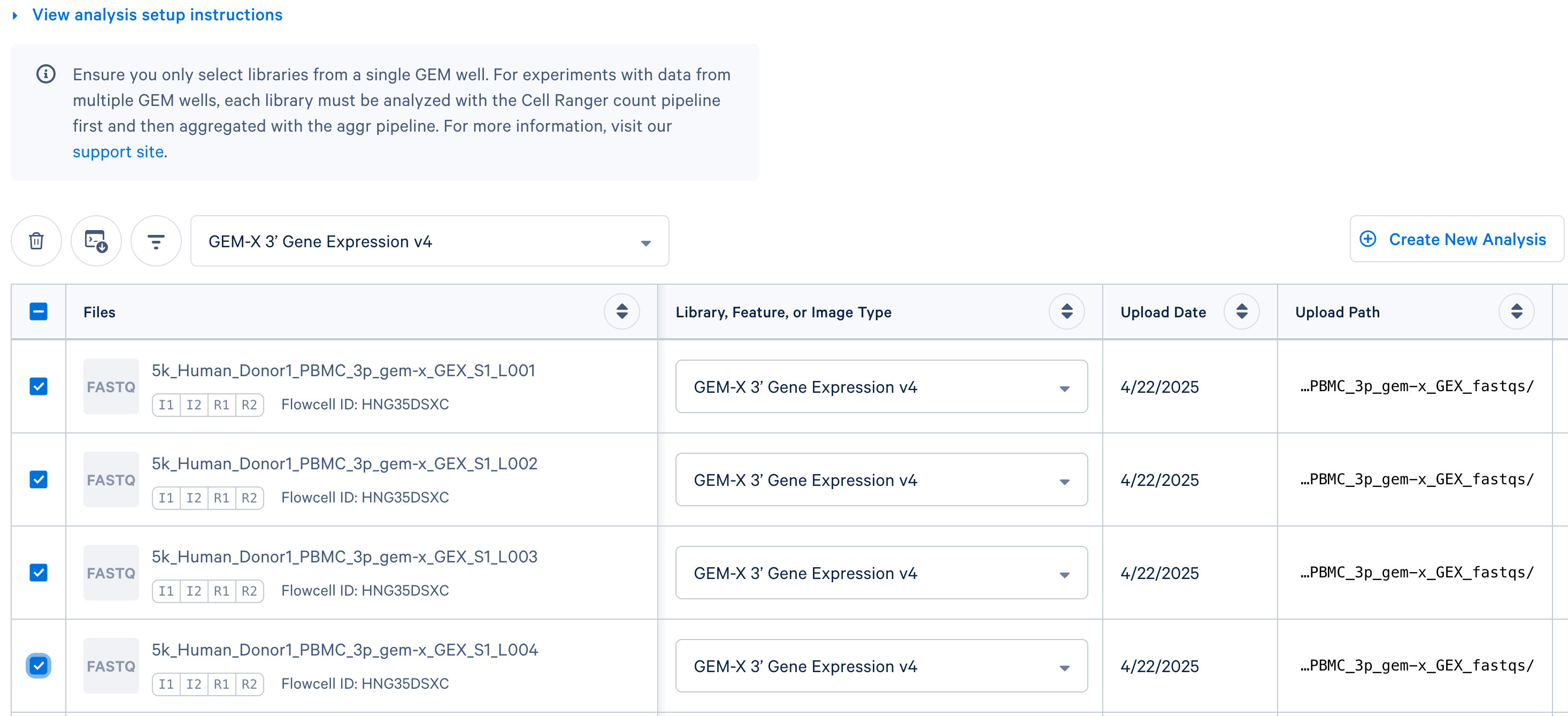
3. Select the "Library Type" for the FASTQ files. For the example datasets, the library type would be "GEM-X 3' Gene Expression v4".

   
   
   

4. To create an analysis to process the reads, select the FASTQ files from the same GEM well. The four GEM-X PBMC datasets used in this tutorial are from separate GEM wells, so we will create four analyses, one per sample.

5. Set up the analysis by following the prompt. When processing FASTQ files for the first time, we do not recommend changing default settings. You may revisit the analysis setup later if the analysis fails or unexpected issues arise in the quality control step.

   
   
   

Obtain output files from the analysis

Once the analysis has been completed successfully, you can download the output files directly through your web browser, as described on this page. The output structure and files of the Cell Ranger multi pipeline are explained on Outputs of Singleplex Library Analysis. Key files are located under "Per sample outputs" and include:

• Summary HTML (web_summary.html): An interactive HTML file providing a visual summary of the data quality. We will use this file for data quality assessment.
• Loupe Browser File (sample_cloupe.cloupe): A file for use with Loupe Browser, enabling detailed exploration of the single cell data and cell type annotation results. We will use this file for data quality assessment, barcode filtering, and as input for downstream analyses.
• Feature / cell matrix (sample_filtered_feature_bc_matrix and sample_raw_feature_bc_matrix): Directories containing the count matrices with genes as rows and cell barcodes as columns, both for the filtered and raw gene expression data. These are often taken as input by community-developed tools for specialized analyses.

After processing your raw data with the Cell Ranger multi pipeline, the next step is to assess data quality and filter out low-quality cells before moving on to downstream analyses. There are several strategies to achieve this, and below we outline recommended practices and diagnostic tools for 10x single cell RNA-seq data. As a best practice, it is recommended to perform QC and barcode filtering on each sample individually before proceeding with data integration and downstream analyses.

The Cell Ranger multi pipeline generates a web_summary.html file, which provides an overview of the analysis performed on the data. It is highly recommended that you review this report as a first-pass QC check for each sample. Review this page for a detailed walkthrough of different views and tables in the web summary file. While some quality issues can be addressed bioinformatically (detailed in the next section), others reveal critical experimental flaws. Such severe flaws (e.g., loss of single cell behavior) often require troubleshooting the experiment itself, as bioinformatic approaches alone may not suffice.

Below is a screenshot of the Gene Expression view in the web_summary.html file from one of the GEM-X PBMC example datasets. This view contains critical metrics and plots to assess the quality of the Gene Expression library.

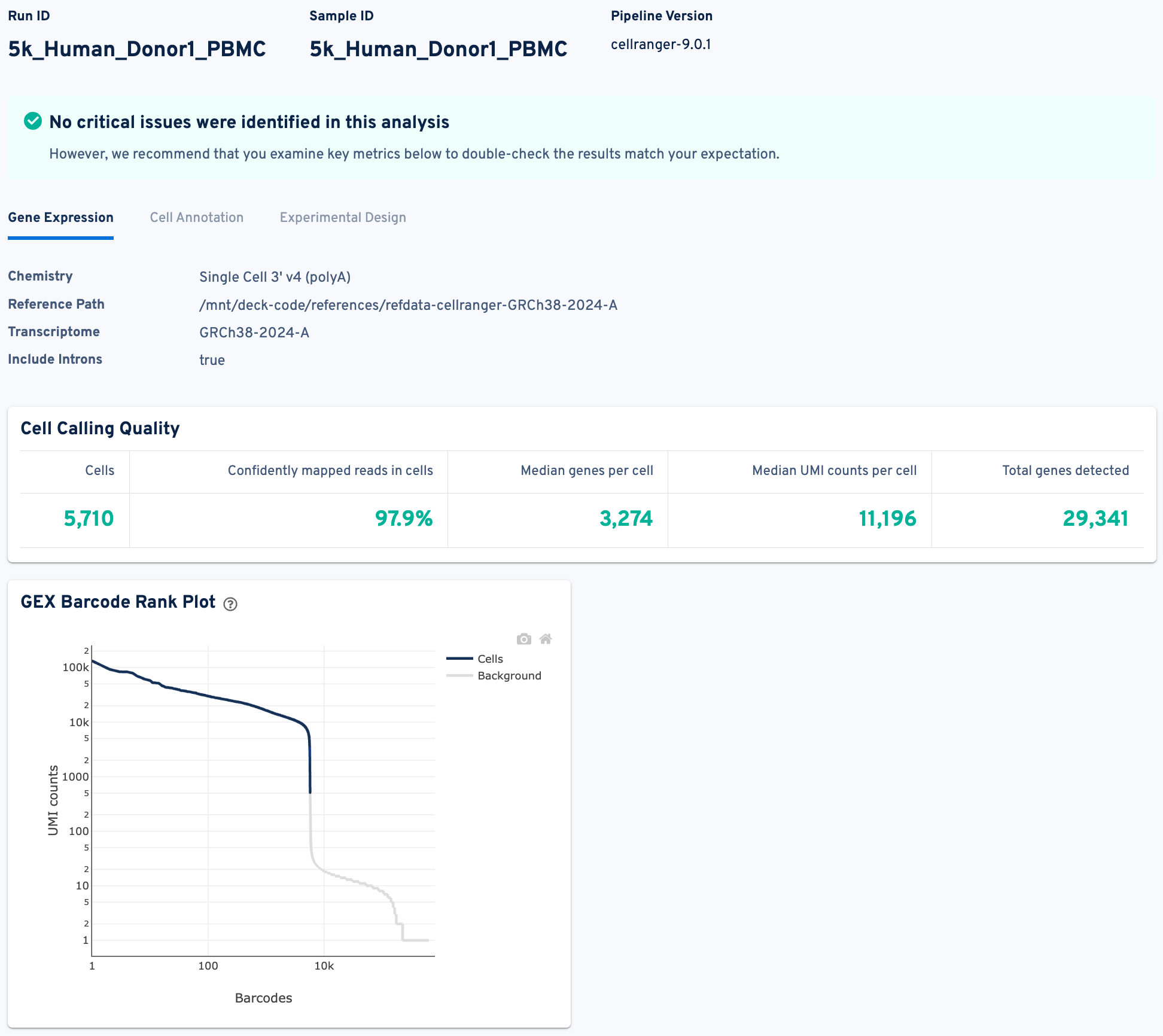
We will not delve into every detail of this report here, as comprehensive explanations for each metric are available in our documentation. Notably, the green message at the top, "No critical issues were identified in this analysis", and the absence of any alert messages, indicate a good starting point for our data. Most metrics in the Cell Calling Quality table align with our expectations for a successful run.

• For instance, the number of cells recovered is 5,710, which is close to the targeted 5,000 cells for this particular sample.
• The percentage of "Confidently mapped reads in cells" is high at 97.9%, and the "Median genes per cell" (3,274 for this sample) is within the expected range for PBMC samples.
• Furthermore, the Barcode Rank Plot displays a characteristic "cliff-and-knee" shape, which is indicative of good quality separation between cells and background.

As a general best practice, always remember to thoroughly examine all other metrics, including mapping and sequencing quality metrics, to ensure there are no obvious issues with the data. For a detailed guide on interpreting each metric and plot for gene expression data, see this tech note.

After the initial QC using the web summary file, you can perform further data exploration and filtering by opening the Loupe file (generated by cellranger multi) in Loupe Browser. Loupe Browser is an interactive desktop software that provides the intuitive functionality you need to explore and analyze your 10x Genomics Chromium data. In the Loupe filtering and reanalysis flow, we can visualize the data distribution and filter out potential low-quality cells based on commonly used QC metrics. To ensure future reproducibility, remember to document the filtering thresholds used.

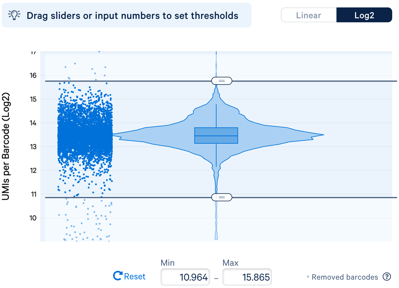
a. Filtering cell barcodes by UMI counts: The total UMI counts associated with a cell barcode represent the number of observed transcripts in the droplet. Barcodes associated with unusually high UMI counts might be multiplets (i.e., one droplet containing multiple cells), whereas barcodes with low UMI counts might be droplets containing ambient RNAs but not real cells. Therefore, using UMI counts to filter cell barcodes may help eliminate barcodes that do not represent a single cell.

As an example, below is the UMI distribution of cell barcodes in the donor 1 dataset. You can drag the slider to set the filtering thresholds. In this example, the extreme outliers with very high and low UMIs will be removed.

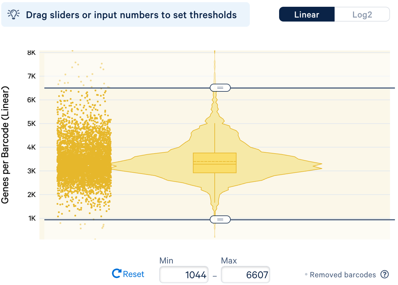
b. Filtering cells by number of features: Similar to the observation with UMI counts, barcodes associated with unusually high number of features might be multiplets, whereas barcodes with low number of features might be droplets containing ambient RNAs but not real cells.

For the example datasets, we will remove the extreme outliers with very high and low number of features in the distribution, similar to the approach taken for the filtering by UMI counts.

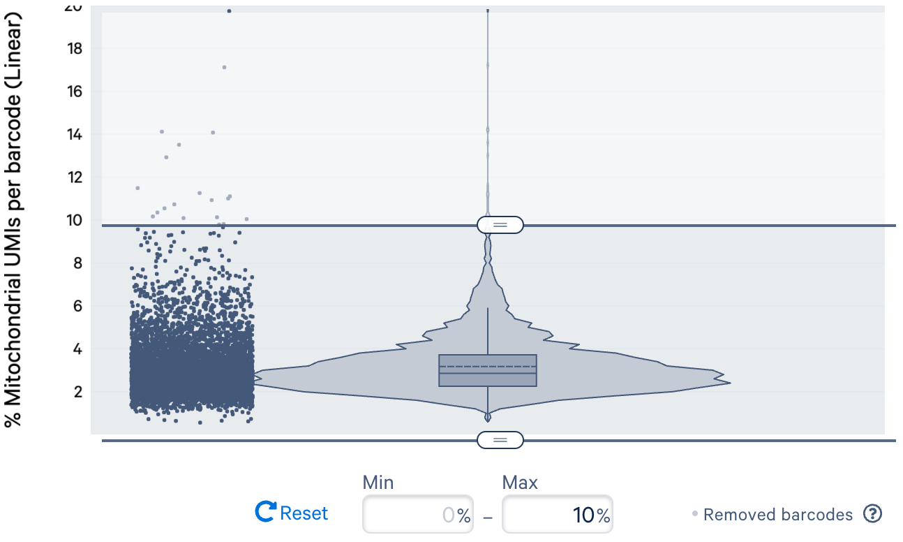
c. Filtering cells by percent of mitochondrial (mt) reads: An increased level of transcripts from mt DNA in cells has been associated with unhealthy cell states or a result of broken cells where the cytoplasmic RNAs leaked out of the cell while the mt RNAs retained in mitochondria are captured in the assay. It is worth noting that the expression level of mt genes can vary among samples. For some cell types (e.g., cardiomyocytes), expression of mt genes may have biological meaning and filtering cell barcodes based on mt reads may lead to bias in the analysis.

High mitochondrial gene expression is not expected in our example PBMC datasets. For instance, in the donor 1 dataset, since most cell barcodes exhibit fewer than 10% UMI counts from mitochondrial genes, we use 10% as the filter threshold for this specific dataset.

The diagnostic plots and QC filters discussed in the previous section are essential for initial data assessment and allow for manual identification of low-quality barcodes. Here we briefly discuss two additional, optional computational approaches that may serve as alternatives or complements to manual methods. The decision to employ these advanced techniques typically depends on your dataset's characteristics and analytical goals.

Ambient RNA removal: This approach addresses contamination from free-floating RNA released by lysed cells during sample preparation. Ambient RNA correction tools aim to estimate the profile of this background noise and computationally remove its contribution from the gene expression counts of genuine cells. This can be important when looking for subtle expression patterns or rare cell types whose marker genes might also be present at low levels in the ambient pool. Commonly used tools include SoupX and CellBender. 10x Genomics also has a couple of analysis guide articles on this topic:

• Introduction to Ambient RNA Correction
• Background Removal Guidance for Single Cell Gene Expression Datasets Using Third-Party Tools

Algorithmic Doublet Detection: This approach identifies droplets containing two or more cells, which create artificial mixed transcriptomic profiles. Manual review of diagnostic plots (as discussed previously) is often a sufficient initial method, particularly for new users or clear signals. For subtle cases or advanced workflows, algorithmic tools offer complementary, computational doublet flagging and can be explored for deeper analysis. Commonly used tools for this purpose include scDblFinder and DoubletFinder.

For the analyses in this article, we will skip these two optional steps as the primary quality control measures already applied are sufficient to illustrate the key analytical concepts covered in this article.

Normalization is a critical step in single cell RNA-seq analysis because raw UMI counts are influenced by a number of technical factors that can obscure true biological signals, including differences in capture and reverse transcription (or probe hybridization) efficiency, variation in sequencing depth, etc. Here, we will use the SCTransform method from the Seurat package, available on the 10x Cloud, to normalize multiple samples. SCTransform is a commonly adopted normalization approach in the literature and performs three major functions:

1. Normalizes data by modeling counts as a function of cell-specific sequencing depth
2. Stabilizes the variance by calculating Pearson residuals from the model, making the variance in normalized counts due to technical factors comparable across genes
3. Identifies highly variable features based on the variance of the Pearson residuals

For details about the algorithm behind SCTransform, see this publication.

To perform normalization using SCTransform on 10x Cloud, we will select the "Normalization (SCTransform) and batch correction (Harmony) workflow". 10x Cloud and Cell Ranger provide another approach to normalization and batch effect correction with the aggr pipeline. Learn more about which to choose here.

This workflow requires individual Loupe (.cloupe) files from individual samples as input. For uploading Loupe files and initiating the analysis workflow, see instructions here. For this step, we will skip the batch correction (Harmony) component within the workflow, by toggling the option "skip batch correction" on when setting up the analysis.

This approach is particularly advisable if you are merging the datasets for the first time or are uncertain about the extent of potential batch effects. A discussion on identifying and addressing batch effects, including the functionality of Harmony, will be provided in a later section.

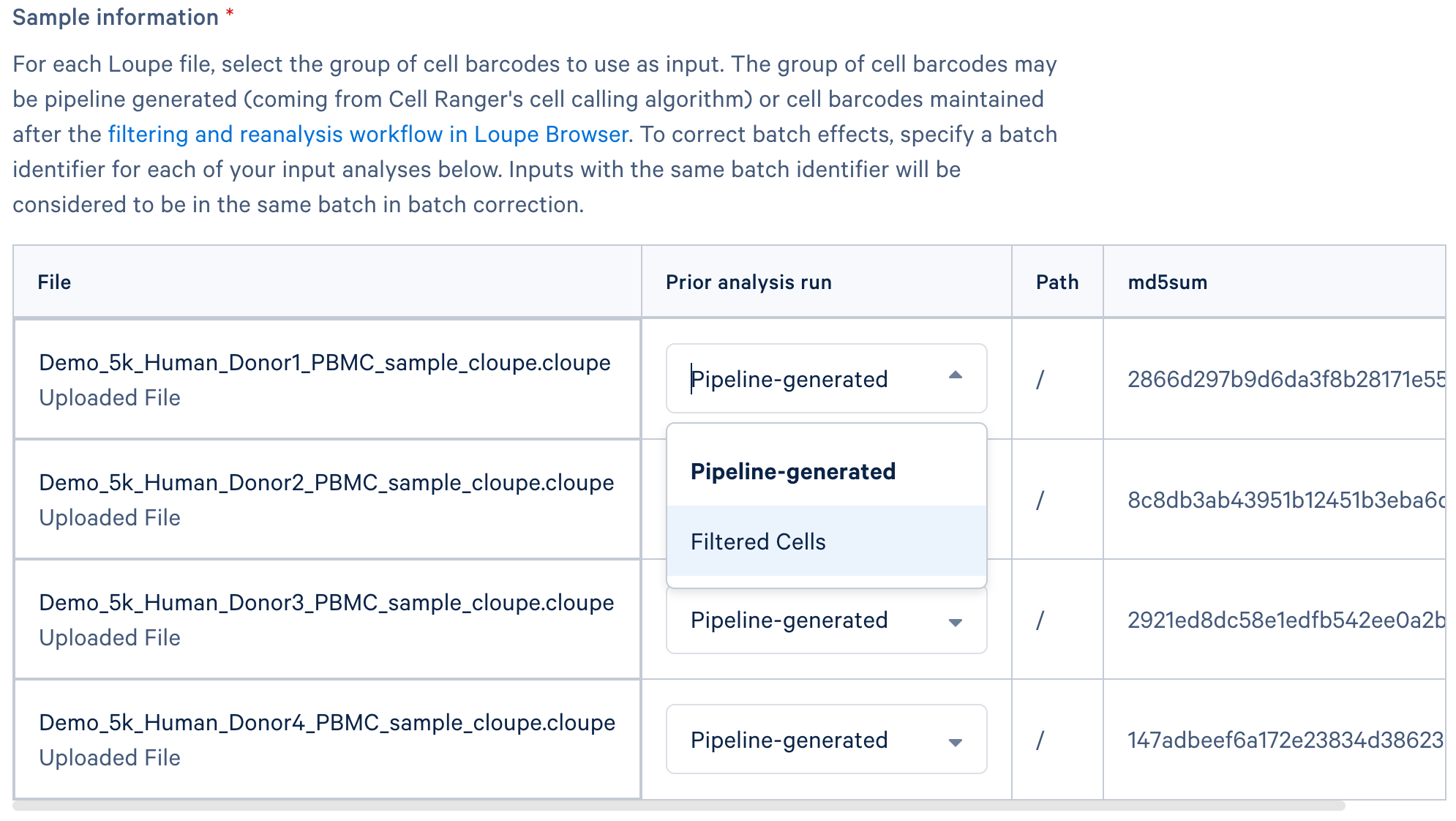
A key feature in this workflow on 10x Cloud is the ability to specify the set of cell barcodes for normalization, allowing you to use the set of cells from upstream quality control and filtering in the Loupe file (e.g., "Filtered Cells" in the screenshot below) instead of all cell barcodes detected by Cell Ranger ("Pipeline-generated").

After normalizing and merging data from multiple samples, the workflow performs cell type annotation (discussed in a later section). It then outputs an integrated_cloupe.cloupe file containing the merged and annotated data from all input samples, ready for further exploration. For details on the outputs from this workflow, see this Expected outputs table.

For alternative normalization methods in the community, see this Single-cell RNA-seq Data Normalization guide.

Single cell RNA-seq data typically comprise expression levels for thousands of genes across thousands of cells. However, interpreting this high-dimensional space directly is difficult, and the inherent sparsity and technical noise in individual gene measurements can obscure underlying biological signals. Dimensionality reduction is therefore a standard step in single cell analysis because it enhances visualization by projecting the data into two or three dimensions, and often consolidates information across genes to provide more robust, less noisy representations. For single cell RNA-seq data, three methods are commonly used for dimensionality reduction.

1. Principal Component Analysis (PCA): PCA is a linear dimensionality reduction method that finds a new set of uncorrelated variables—called principal components (PCs)—which capture the maximum variance in the data. PCA is widely used in single cell analysis as an initial denoising and data-compression step. It reduces complexity and is typically used to generate inputs for further nonlinear methods (e.g., t-SNE or UMAP). It does not appear in the Loupe file because it is the initial step of dimensionality reduction and is not commonly used for visualization of cell clusters in single cell data.
2. t-Distributed Stochastic Neighbor Embedding (t-SNE): t-SNE is a nonlinear method optimized for visualizing high-dimensional data in two or three dimensions by preserving local relationships between cells. t-SNE is excellent at preserving local (neighborhood) structure. However, it may distort global relationships, making distances between clusters difficult to interpret.
3. Uniform Manifold Approximation and Projection (UMAP): similar to t-SNE, UMAP is a nonlinear method optimized for visualizing high-dimensional data in two or three dimensions. UMAP is generally faster than t-SNE and can scale better with larger datasets. It often produces embeddings that appear to better represent the global arrangement of clusters.

For details on how Cell Ranger performs dimensionality reduction, see this section on our support site. We will use the computed UMAP projections (from the normalization step on 10x Cloud), already present in Loupe files, for data visualization in the subsequent steps.

Clustering is a fundamental step in analyzing single cell RNA-seq data, typically performed after data normalization and dimensionality reduction. The objective is to computationally group cells with similar gene expression profiles. These groups, or clusters, often correspond to distinct cell types, subtypes, or cellular states present in the original sample. By partitioning cells into meaningful clusters, researchers can better understand the cellular heterogeneity within their data.

When working with Loupe files, the clusters from graph-based and K-means clustering are computed by Cell Ranger or the "Normalization (SCTransform) and batch correction (Harmony) workflow" on the cloud.

Graph-based clustering

For scRNA-seq data, the most effective and widely used clustering strategies are graph-based methods, particularly those employing a Shared Nearest Neighbor (SNN) approach. This methodology is well-suited to the high-dimensional and sparse nature of single cell transcriptomics data, offering key advantages over traditional algorithms like K-means.

• K-means typically assumes clusters are spherical. Graph-based clustering, however, can better identify clusters that are complex and not necessarily round.
• Unlike K-means, graph-based clustering determines cluster numbers from the data's structure, not from a user-predefined number.

These robust characteristics and practical benefits explain why graph-based clustering is the default clustering method in widely used toolkits like Seurat (FindClusters function) and 10x Genomics' Cell Ranger software (output in the Loupe file).

K-means clustering

Cell Ranger also performs K-means clustering and the clusters can be explored in the Loupe Browser. K-means is a classic clustering algorithm that partitions data into a user-specified number (k) of clusters by minimizing the distance between cells and the centers (centroids) of their assigned clusters. While graph-based clustering is often preferred for defining final cell populations, the simpler K-means algorithm can be useful in initial data assessment.

Using a small k (e.g., 3-5), K-means provides a rapid overview of major cellular divisions. For instance, differential expression analysis between these broad clusters can identify marker genes for each. These markers can then help assign preliminary, high-level cell type annotations (e.g., immune, stromal, epithelial cells) to the major populations in the data.

Separately, K-means can quickly assess if predefined experimental groups (e.g., diseased vs. normal, treatment vs. control) segregate into distinct clusters. This outcome can indicate if the condition is a strong driver of global transcriptional differences.

K-means may also be useful when k is confidently known beforehand (e.g., expected number of cell populations), or for clustering specific cell subtypes within a well-defined cell population.

After clustering cells, DE analysis identifies genes that are significantly up- or downregulated in each cluster compared to others. These marker genes define the molecular signature of each cluster, bridging the gap between computational grouping and biological interpretation. Note that this approach is excellent for defining the identity and unique molecular signatures of each cluster but does not inherently compare biological conditions across replicates.

Both Cell Ranger and Loupe Browser can perform DE analysis for cluster characterization. For the algorithm details, see this section on our support site. In short, for each gene and each cluster i, Cell Ranger tests whether the mean expression in cluster i differs from the mean expression across all other cells.

As discussed in the previous section, DE analysis can be applied to those broad K-means clusters to help characterize major cellular divisions in the data. In addition, DE analysis is an excellent method for performing a preliminary check on automated cell type annotations, ensuring they align with underlying gene expression patterns and known biology.

Here, we use the cell annotations from our integrated_cloupe.cloupe file, generated from 10x Cloud in an earlier step (Normalization and data merging). We perform DE analysis using Loupe Browser, treating each annotated cell type as a distinct group (or "cluster").

The goal is to identify upregulated genes for each annotated cell type, which are the primary DE analysis results we will use. In the next section, we compare these genes to known markers (from literature/databases) to evaluate the biology of the annotations and identify any that require further investigation.

Cell annotation assigns a biological label to each group of cells in the data, and is key to interpreting the cellular composition of your samples.

Both Cell Ranger (starting from v9.0.0) and the data integration pipeline on the 10x Cloud can perform reference-based automated cell annotation on human and mouse datasets, which you can explore in Loupe Browser. For the details of the algorithm and reference data, see Cell Ranger's Cell Annotation Algorithm.

Automated cell type annotation provides a valuable starting point, but these initial assignments should be reviewed and may need to be refined. For each assigned cell type, check its top marker genes identified through differential expression (DE) analysis. Do these markers match known, canonical markers for the assigned cell type? For example, if a cluster is labeled "B cells", you should expect to see high expression of markers like CD19, MS4A1 (CD20), or CD79A in its DE gene list. Discrepancies may indicate inaccurate annotations, novel cell states, or the presence of finer-grained cell subtypes.

In this section, we will demonstrate how to evaluate the cell annotation results using two approaches in Loupe Browser.

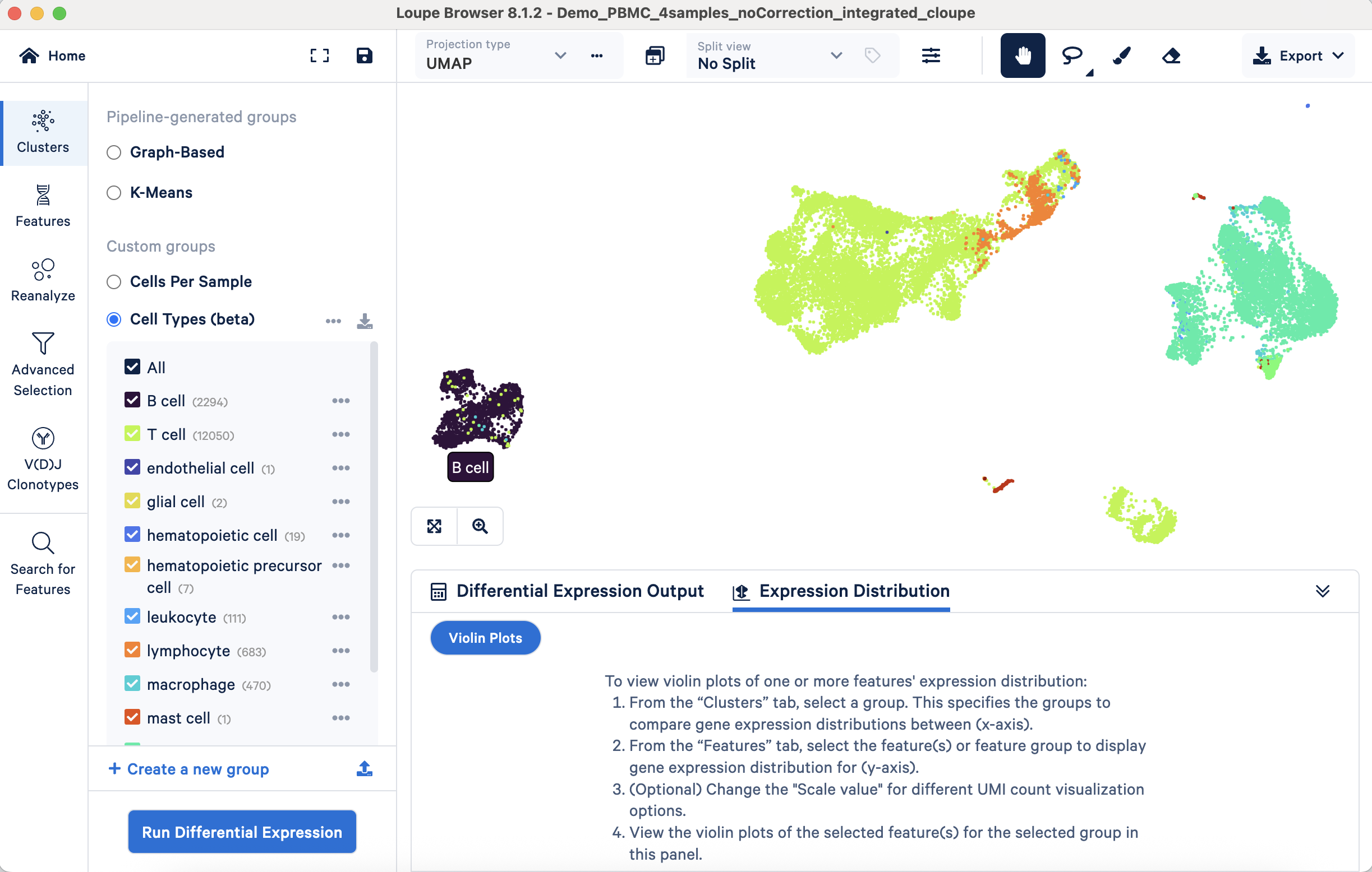
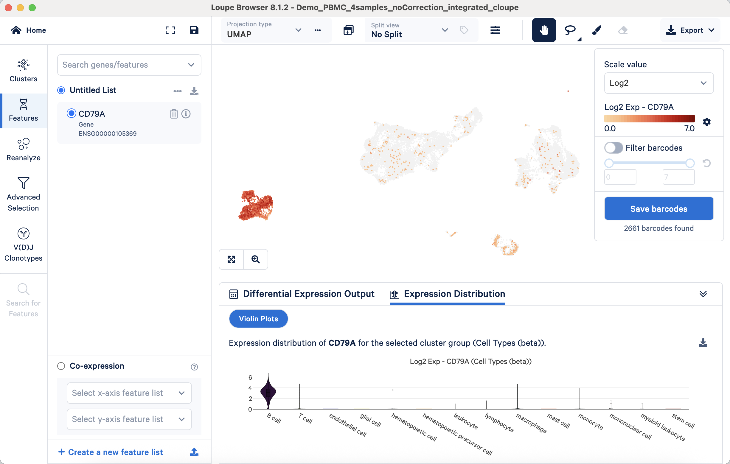
• Approach 1: Validating annotations with marker gene expression through visualization. This approach verifies whether known marker gene expression aligns with annotated cell populations. For example, the B cell marker CD79A's expression should be predominantly observed on the UMAP projection within the annotated B cell cluster. Correspondingly, violin plots should confirm its largely exclusive expression in B cells compared to other cell types:

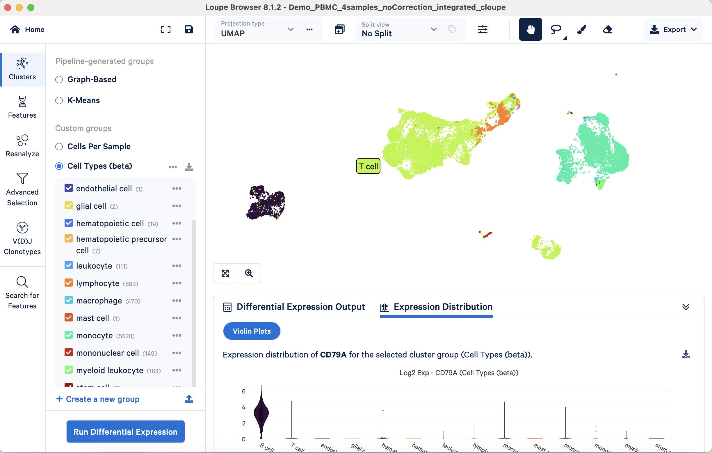
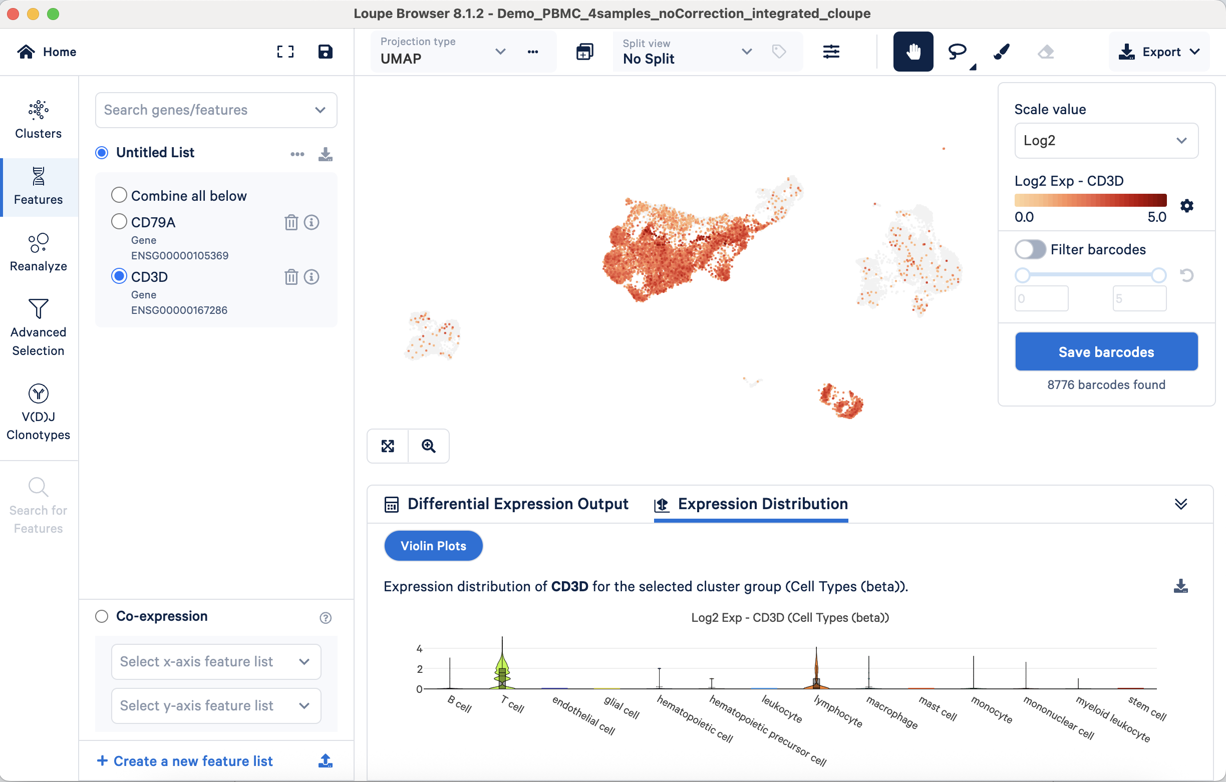
Similarly, the T cell marker CD3D should show predominant expression within the T cell population across these visualization types:

This validation process can be systematically applied to all annotated populations using their respective markers. This approach is also useful for refining broader annotations such as "lymphocyte" or "leukocyte", to further delineate constituent subpopulations.

• Approach 2: Validating annotations with differential gene expression analysis. This approach uses the result from Loupe Browser's DE analysis (performed in the Differential expression analysis for cluster characterization section) to validate cell annotations. The list of genes significantly upregulated in an annotated cluster should prominently feature established markers for that cell type. For instance, as shown in the screenshot below, canonical B cell markers such as CD79A and MS4A1 (CD20) are identified as top upregulated genes in the B cell population.

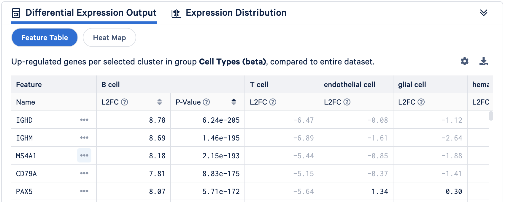
Similarly, key T cell markers like CD3D and CD3E are also found to be significantly upregulated in the annotated T cell population. The presence of these characteristic markers in the significantly upregulated gene lists provides strong support for the assigned cell identities.

Manual cell type annotation relies on biological expertise to interpret clustering and gene expression data. For this purpose, the expression profiles of each cluster are compared to all other clusters to identify the differentially expressed genes. Carefully examine the top marker genes for each cluster and consult literature and cell marker databases (see examples in this article) to identify cell types known to express those specific combinations of markers. Then, assign a cell type label to each cluster based on this evidence.

Manual annotation can be used independently or, more commonly, to validate, refine, or correct the initial assignments from automated methods. While more time-consuming, it allows for nuanced interpretation and identification of potentially novel cell states not present in reference datasets. Although manual annotation is a valuable technique, we will omit it in this tutorial to focus on the automated results, which provide a sufficient basis for our evaluation. See this page for a tutorial on how to perform manual cell type annotation.

Beyond the integrated 10x Genomics tools, the broader bioinformatics community has developed numerous popular tools for automated cell type annotation, often used in R or Python environments. Some popular tools include Azimuth, SingleR, and CellTypist. If alternative automated annotation is desired, you may use the Seurat object or integrated feature-barcode matrix from the "Normalization (SCTransform) and batch correction (Harmony) workflow" (on 10x Cloud) as input for community-developed tools.

When analyzing data from multiple single cell experiments, especially those processed at different times or under slightly different conditions (different sequencing runs, library preparations), technical variations known as "batch effects" can arise. These systematic, non-biological differences can confound downstream analysis, making it crucial to diagnose and, if necessary, correct for them. Separately, batch correction methods can be used for "data harmonization", such as in cell atlassing to identify consistent cell types across samples (e.g., patients), where each sample is often treated as a "batch".

Before applying any correction, it is essential to determine if significant batch effects exist in your integrated dataset.

• Visual inspection: After initial data normalization (SCTransform) and merging on 10x Cloud, you can open the merged Loupe file in Loupe Browser. There will be a Custom group called "Cells Per Sample", which colors the UMAP plot by sample:

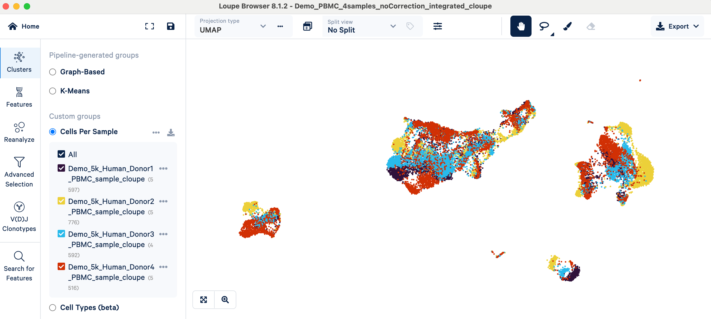
• Interpretation: If cells cluster predominantly by their batch of origin (or in our example, by donor/sample) instead of by expected biological cell types, a batch effect is likely present. In the PBMC example, you can see cells annotated with the same cell type (e.g., T cells, see screenshot above) forming separate clusters simply because they originated from different donor samples. This indicates that batch correction may be needed so that the clustering can represent meaningful biology instead of technical variability between samples.
• Caution: Be mindful if your biological condition of interest perfectly correlates with batch (e.g., all control samples are in batch 1, all treatment samples are in batch 2). While correction methods can still be applied, interpreting the results requires extra care, as distinguishing true biological effects from technical batch effects becomes inherently more challenging.

If batch effects are detected, you can go back to the data integration pipeline on 10x Cloud to perform normalization followed by batch correction by enabling batch correction (default) this time. The batch correction method used in the pipeline is Harmony, which has been identified as a high-performance batch correction technique in benchmarking publications (Tran et al., 2020, Antonsson & Melsted, 2024). For details about the algorithm behind Harmony, see this publication. Harmony operates on the reduced-dimensional representation of the data (typically the PCA coordinates), and then recomputes the integrated embedding. The corrected UMAP can be visualized in the integrated Loupe file.

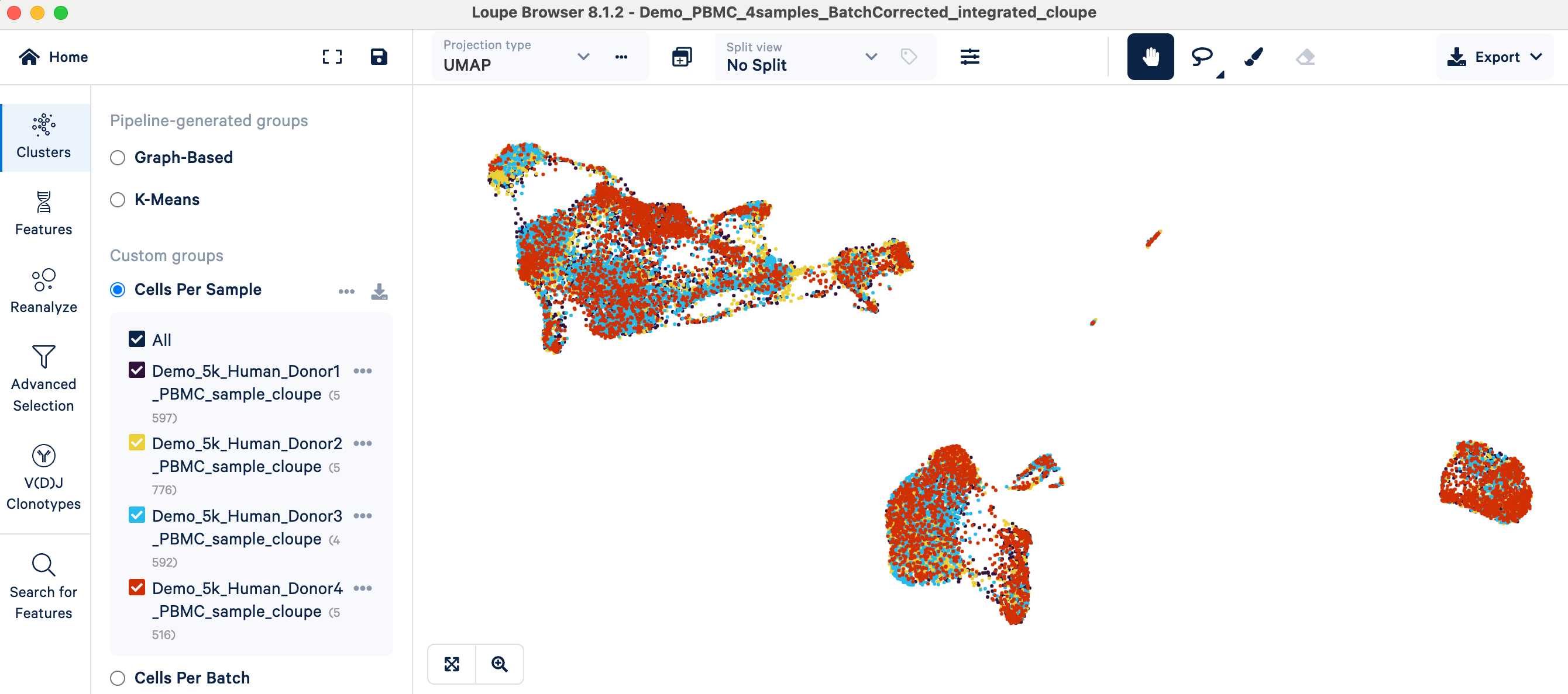
For example, using the four healthy PBMC datasets from four different donors, after applying Harmony batch correction via the "Normalization (SCTransform) and batch correction (Harmony) workflow" on 10x Cloud, the resulting UMAP shows that the distinct, sample-specific clusters observed before correction are now well mixed. Cells of the same type (e.g., T cells) from the four different donors now co-cluster, indicating that the technical variability due to batch effects has been successfully corrected:

• Changed: Downstream visualizations (UMAP/t-SNE plots) generated from the corrected embeddings will show better integration (mixing) of cells from different batches. The resulting cluster definitions will also reflect the batch-corrected structure. This is crucial for reliable subsequent analyses. For instance, differential expression analysis becomes more accurate—despite Harmony not changing gene counts—by operating on cell clusters that better represent distinct biological groups.
• Unchanged: Harmony does not alter the underlying UMI counts in the feature-barcode matrix. The raw counts and the values derived from normalization methods like SCTransform remain untouched by the Harmony integration process itself.

While we do not expect automated cell annotations to change after batch correction, you can verify them by reapplying the validation methods described in the cell type annotation section.

While Harmony improves embeddings for visualization and clustering, batch effects arising from technical factors may still impact between-sample DE analysis, which operates on the original matrix instead of an embedding.

The standard method to adjust for batch effects in DE analysis is to include "batch" as a variable (covariate) in a statistical model, i.e., to "correct for batch". If the "batch" variable used by Harmony is a biological variable (e.g., patient ID) instead of a technical variable (e.g., difference in the library preparation), then there is no need to adjust during DE as this is biological signal rather than artifact.

This is performed outside the direct 10x Cloud/Loupe Browser workflow. You can use the integrated matrix.h5 file or the Seurat object output by the integration pipeline as an input for tools like DESeq2 or edgeR to perform such analysis. As this step is optional, in this article we will not consider batches in the cross-sample comparison analysis.

Cross-sample comparison in single cell analysis aims to understand biological similarities and differences by analyzing a combined dataset across various experimental conditions, time points, or biological replicates. A primary goal of this analysis is to uncover unique cell states or cell type-specific responses associated with particular groups of samples.

When performing differential expression (DE) analysis in this context, it is important to utilize methods appropriate for comparing across different samples instead of just identifying cluster markers within a single sample (discussed in a prior section).

For robust cross-sample comparisons, the pseudobulk DE approach is an effective and commonly employed strategy in the literature. This method aggregates gene expression counts per cell type within each sample. These aggregated profiles—each sample providing one data point per cell type per condition—are then used for DE testing between conditions. A key advantage is its proper accounting for biological replication by treating each sample, not each cell, as a replicate. This avoids artificially inflating statistical significance often seen when cells are incorrectly treated as independent replicates across samples, thus ensuring identified differences more reliably reflect true biological changes. The pseudobulk DE approach is utilized by Loupe Browser for multi-sample comparisons, and an example tutorial can be found here.

While Loupe Browser provides a convenient way to perform such analyses, it is worth noting that alternative methods for multi-sample comparison also exist (often performed outside of Loupe), as discussed in this article. For the purposes of this guide, however, we will focus on leveraging the capabilities within Loupe in this section. Specifically, we will use the multi-sample comparison feature in Loupe to compare the PBMC samples from male vs. female donors to identify sex-specific gene expression differences within annotated cell types.

Before setting up the cross-sample DE analysis with the batch-corrected and integrated Loupe file, we need to define the groups (or conditions) for the samples. The steps include:

1. Split the UMAP view by samples
2. Select male samples using the lasso tool
3. Create a new cluster ("Male") and group ("Conditions") name
4. Repeat the above three steps for the female samples. We now have a custom group called "Conditions", containing two clusters - "Male" and "Female".

After the "Conditions" are defined, we can then set up the cross-sample DE analysis:

1. Click "Run Differential Expression"
2. In the Differential Expression Settings, select "Across multiple samples" and start analysis. A new window will open.
3. Select cell types of interest that we want to compare between conditions. For the example analysis, we first select from the group "Cell Types (beta)" (derived from the automatic cell annotation pipeline on 10x Cloud). All the cell types will be populated. While we will keep only B cell, T cell, leukocyte, lymphocyte, macrophage, and monocyte for this demonstration, you should choose the cell types that are pertinent to your own research questions.
4. Select the conditions to perform comparisons. For this analysis, we select from the group "Conditions", and put "Female" as experimental condition A and "Male" as B.
5. Select the corresponding sample IDs for the experimental conditions. For example, here we select from the group "Cells Per Sample", and the sample IDs for each condition populate automatically.
6. Hit the "Run Differential Expression" button.

The analysis will generate lists of differentially expressed genes for each cell type.

As expected, this analysis confirmed that the XIST (X-inactive specific transcript) gene was the most significantly enriched gene in the female group across cell types. This finding is expected because XIST is a well-established, female-specific transcript responsible for X-chromosome inactivation, so its strong and consistent enrichment serves as an excellent positive control. This result validates that the pseudobulk DE analysis is working as intended and able to identify biological differences between sample groups. Users can apply this method to explore more complex biological questions, such as comparing diseased versus healthy cohorts or treated versus control conditions.

Beyond the standard analysis enabled by 10x software tools, several specialized analytical avenues can provide deeper biological insights depending on the specific goals of a study. These often build upon the initial findings and can reveal more complex cellular behaviors and relationships. While a detailed exploration of each is beyond the scope of this guide, we briefly introduce a few common examples, many of which can be performed using the rich ecosystem of community-developed tools.

• Gene Set Enrichment Analysis (GSEA): After identifying differentially expressed genes, GSEA or pathway analysis can help frame these gene lists in a broader biological context. Instead of focusing on individual genes, these methods assess whether predefined gene sets (e.g., those in specific biological pathways) show statistically significant, collective shifts in activity. This can reveal higher-level biological themes obscured when looking at individual genes. Popular tools for this analysis include the original GSEA software from the Broad Institute, the R package clusterProfiler, and fgsea for a fast GSEA implementation.
• Cell-Cell Interaction Analysis: This analysis infers potential communication networks between cell types by examining the expression of ligand-receptor pairs. It helps understand how cells coordinate functions, influence each other, or contribute to tissue homeostasis or disease. Widely used methods include CellChat, which models complex signaling pathways, and CellPhoneDB, which provides a comprehensive repository of ligand-receptor interactions and statistical tools
• Trajectory Inference (Pseudotime Analysis): For dynamic processes like differentiation, trajectory inference orders cells along a "pseudotime" continuum based on gene expression changes, helping to identify genes that vary along the trajectory and characterize intermediate states. Example tools include Monocle 3 and Slingshot. Complementing this, RNA velocity analysis (using tools like velocyto or scVelo) uses unspliced/spliced mRNA ratios to predict short-term cellular state changes, offering a dynamic view of transition direction and speed to refine trajectory models. See the 10x Genomics tutorial for practical application: Trajectory Analysis using 10x Genomics Single Cell Gene Expression Data.

These advanced analyses often require specific experimental designs and leverage a diverse range of powerful computational tools developed by the wider scientific community, enhancing the biological interpretation of single cell RNA-seq datasets.