The Space Ranger-generated clustering and projection analysis contained in a .cloupe file includes all barcodes from tissue-associated spots. However, you may want to only analyze a subset of the clusters, or subregions of interest, or to remove clusters from the analysis.
Loupe v6.3 introduced an interactive filtering and reanalysis workflow for spatial datasets that provides this flexibility. Going through the workflow steps, one can select clusters or regions of interest, filter by UMIs or features, and recompute graph-based clustering, t-SNE, and UMAP projections.
In this tutorial, the concepts associated with reclustering will be demonstrated in a preloaded mouse brain dataset in Loupe Browser.
spaceranger count pipeline. This workflow is not supported for samples processed using spaceranger aggr.- Loupe Browser on macOS or Windows
- Familiarity with Loupe Browser navigation
- Access to tutorial dataset
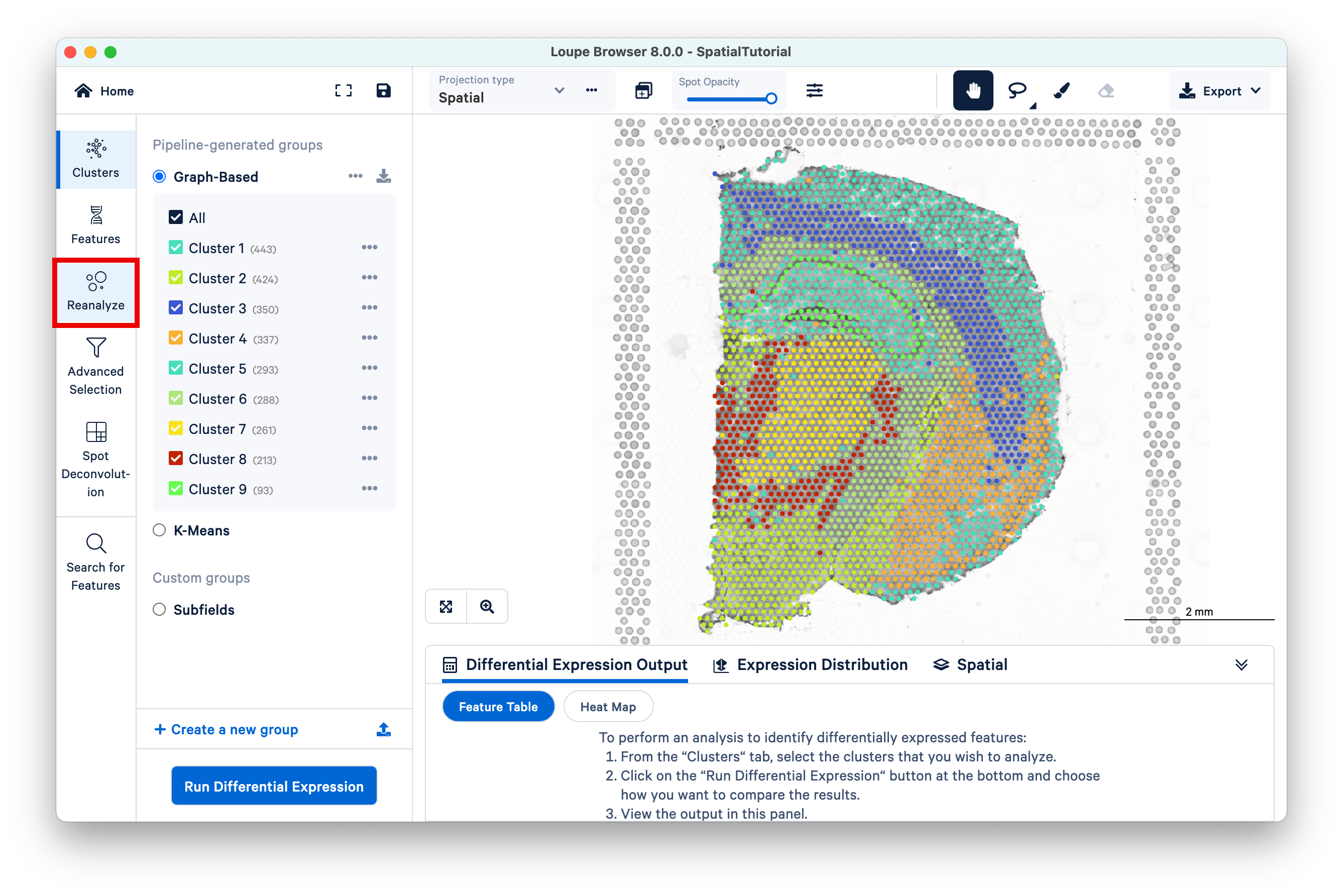
The Recluster workflow can be accessed by clicking Reanalyze on the left.
This opens a new window. Click Got it! to proceed.
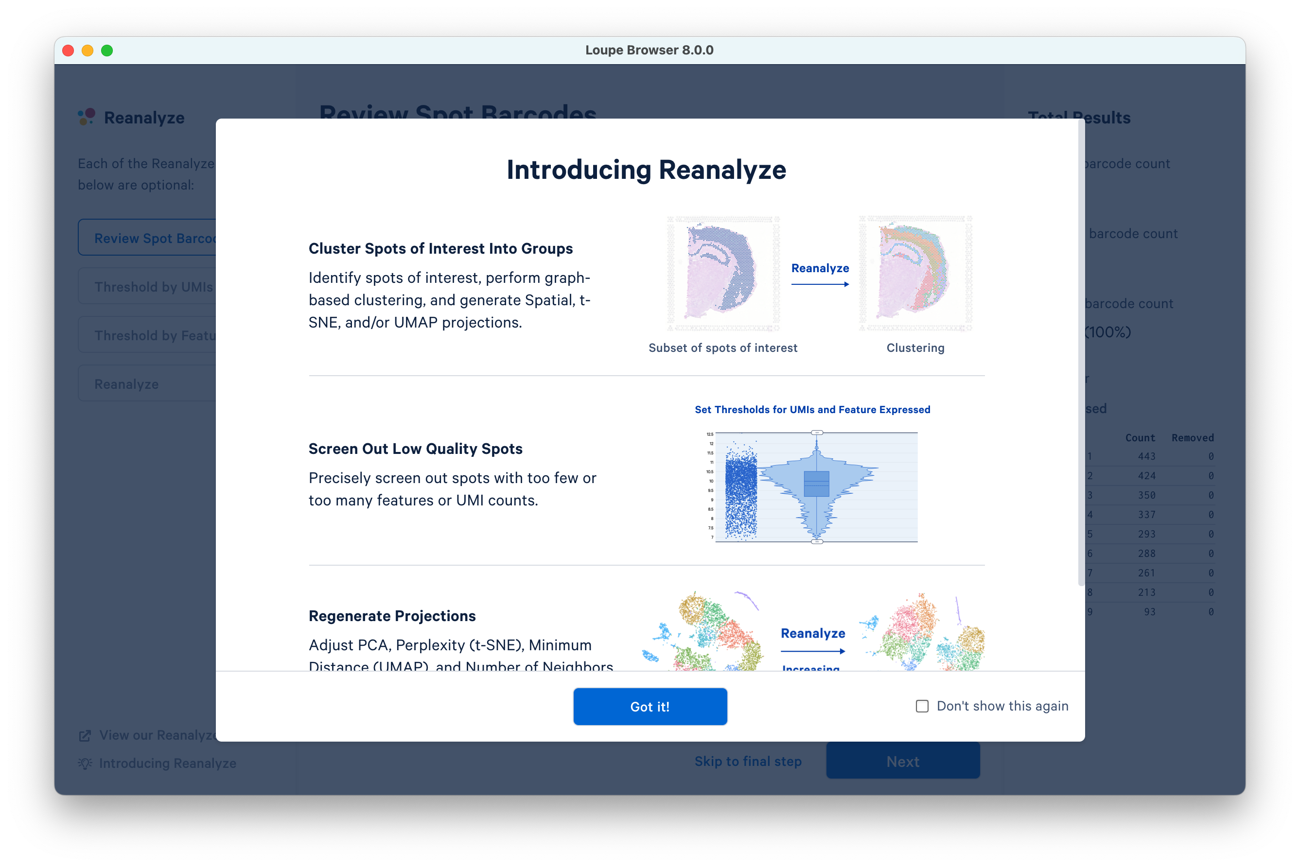
The Reanalyze window consists of three components: the current workflow step on the left, tooling for the active step in the middle, and statistics about the removed barcodes on the right. To progress through each step, click Next. Each step is optional, so you can also Skip to final step.
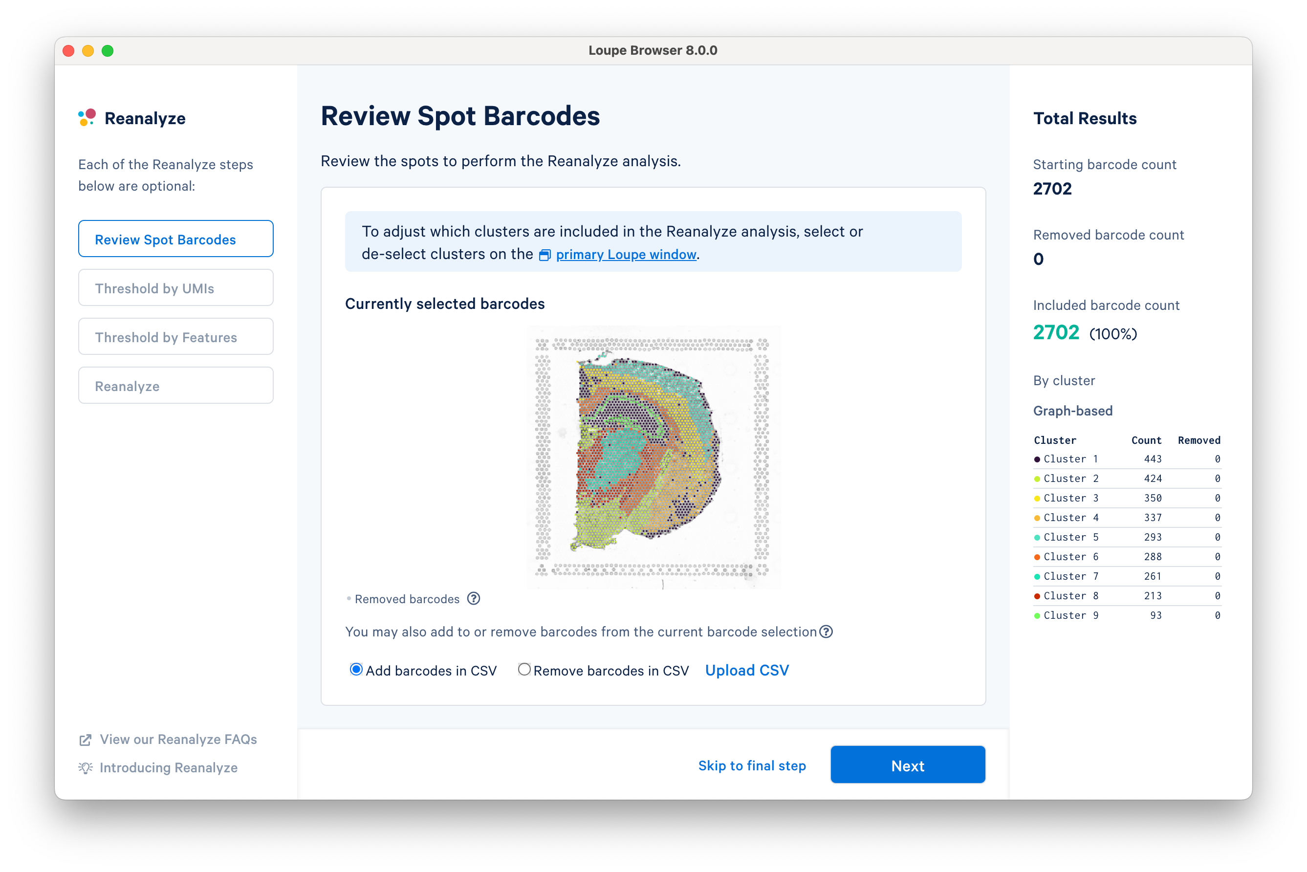
The first step allows initial filtering by cluster selection or a barcode list. The Reanalyze window is linked to the primary window. By default, all the clusters are selected. Changing either the clustering type (Graph-Based, K-Means, or manual) or de-selecting clusters in the primary window is reflected in the reclustering window.
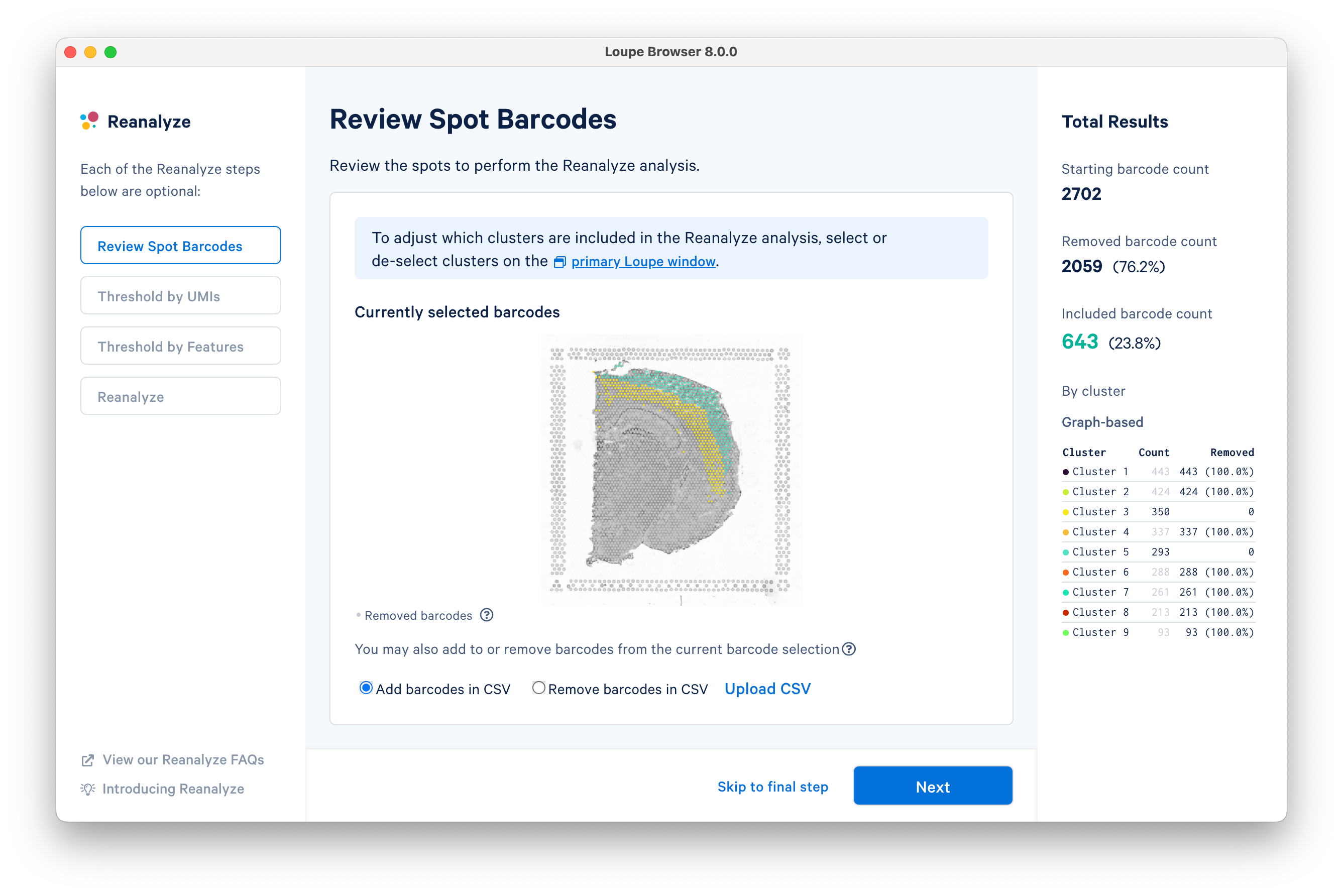
In this tutorial, for the cluster-based selection, clusters 3 and 5 are selected in the primary window. The anatomical region corresponding to these clusters is the isocortex. Subsequently, the reclustering window is automatically updated, listing both the total and per-cluster distribution of the included barcodes.
Reclustering can also be applied to custom categories or regions created using Loupe functions. The customizations can be applied in the main window by creating new categories followed by reclustering, or by importing a CSV file directly using the Upload CSV option. For the former option, it is recommended that the custom categories be created before initiating the reclustering workflow.
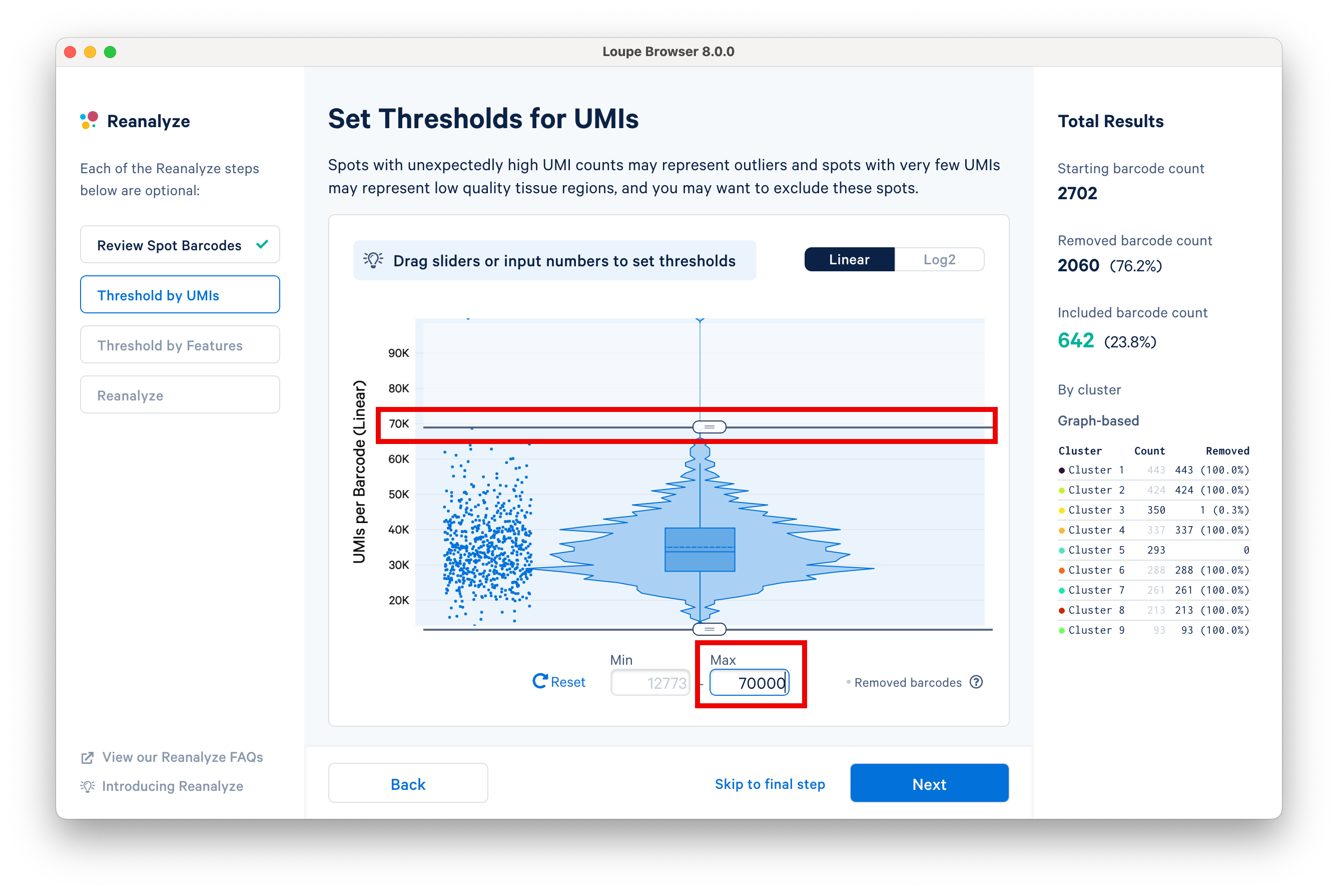
This step allows for filtering by UMI count values for a given barcode or spot for spatial datasets. A violin plot and a box plot of the currently selected barcodes, along with columnar data points for each spot, are shown in the window. By default, the values are shown on linear scale, with an option to view the distribution in log2 scale. Apply the threshold by either moving the sliders on top or bottom of the plot or by manually entering numeric values in the boxes under the plot.
Set an upper UMI count limit of 70,000 UMIs per barcode on the linear scale, and notice that the statistics on the right are updated accordingly.
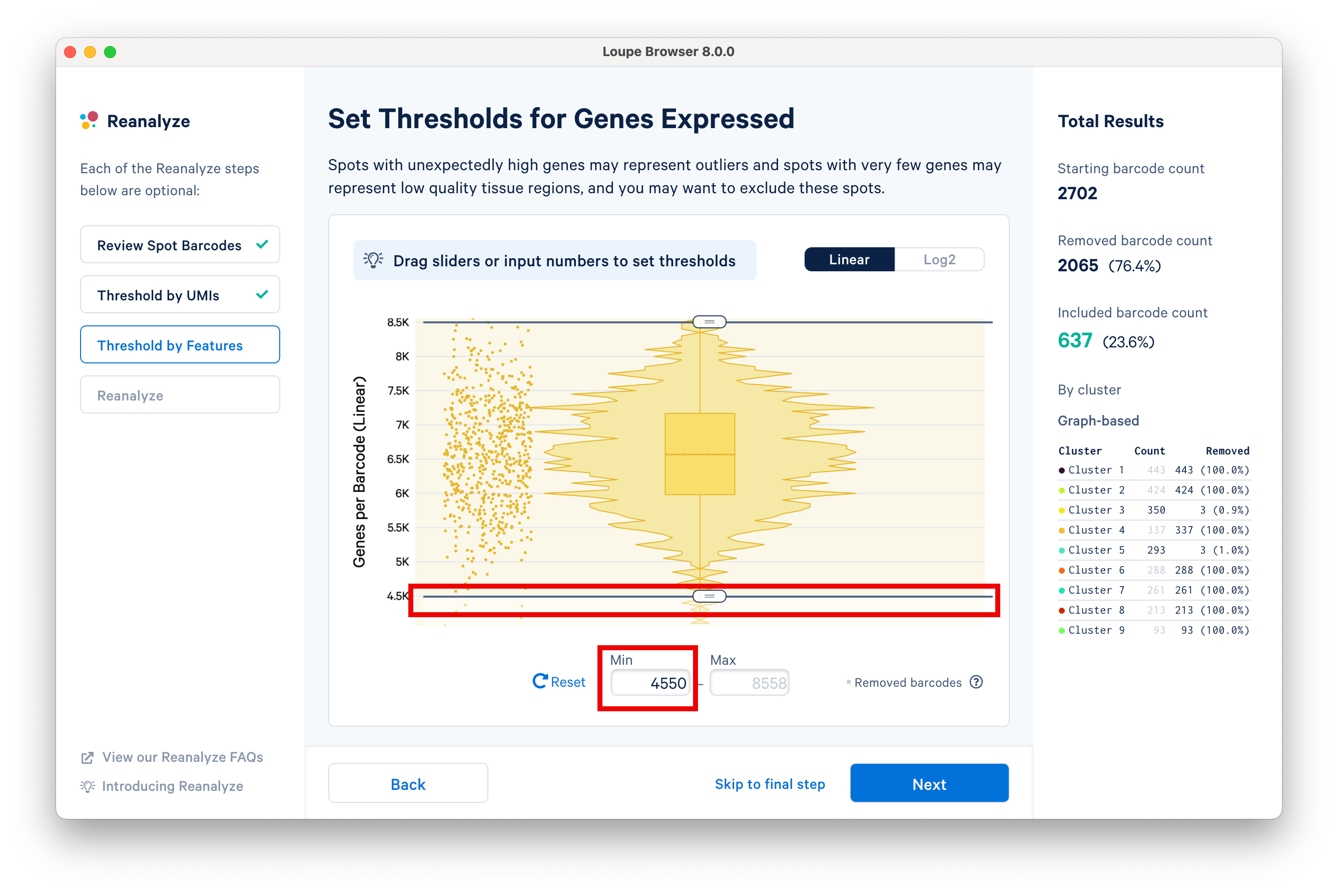
The next step in the workflow allows users to threshold by features. Spots with unexpectedly high genes may represent outliers, and spots with very few genes represent low quality tissue regions. Here, we set the minimum to 4.5K features using the slider.
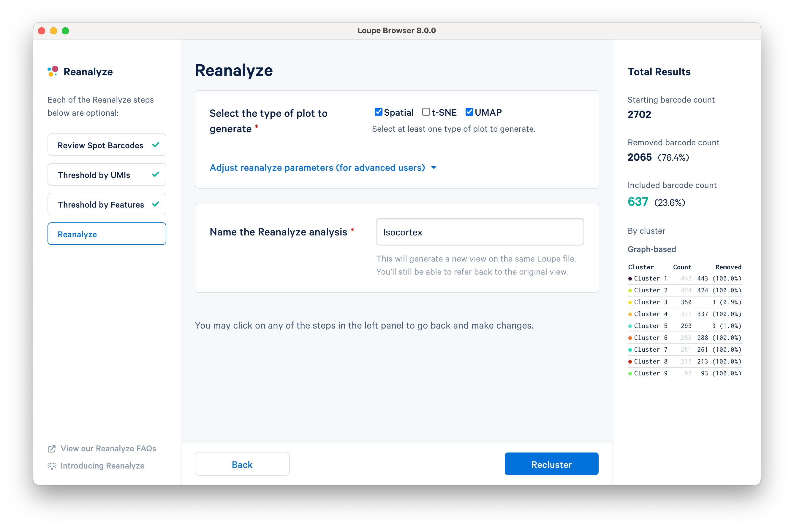
The final step in the workflow allows users to select the type of plot(s) to generate and to fine-tune the plotting parameters. By default, the spatial plot is selected for spatial datasets, with an additional choice of t-SNE and UMAP projections.
The Adjust reanalyze parameters (for advanced users) drop-down menu allows users to change the default parameters for the dimensionality reduction, clustering, and plotting. Click Learn more for additional information about parameter selection.
Name the reclustered dataset "Isocortex". The name will be used in the primary window as both the projection and clustering categories. Adding the name unlocks the Recluster option. Note that duplication of category names from the primary window is not allowed.
Click Recluster to initiate reclustering algorithms. In the background, Loupe will run virtually the same PCA, Louvain clustering, t-SNE, and UMAP algorithms as the Space Ranger pipeline.
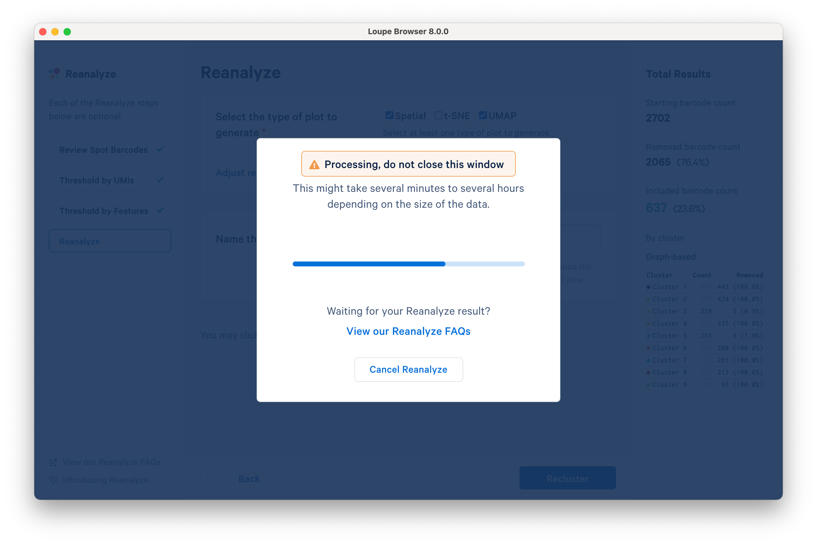
Successful completion of the reclustering workflow will result in updated text on the pop-up window.
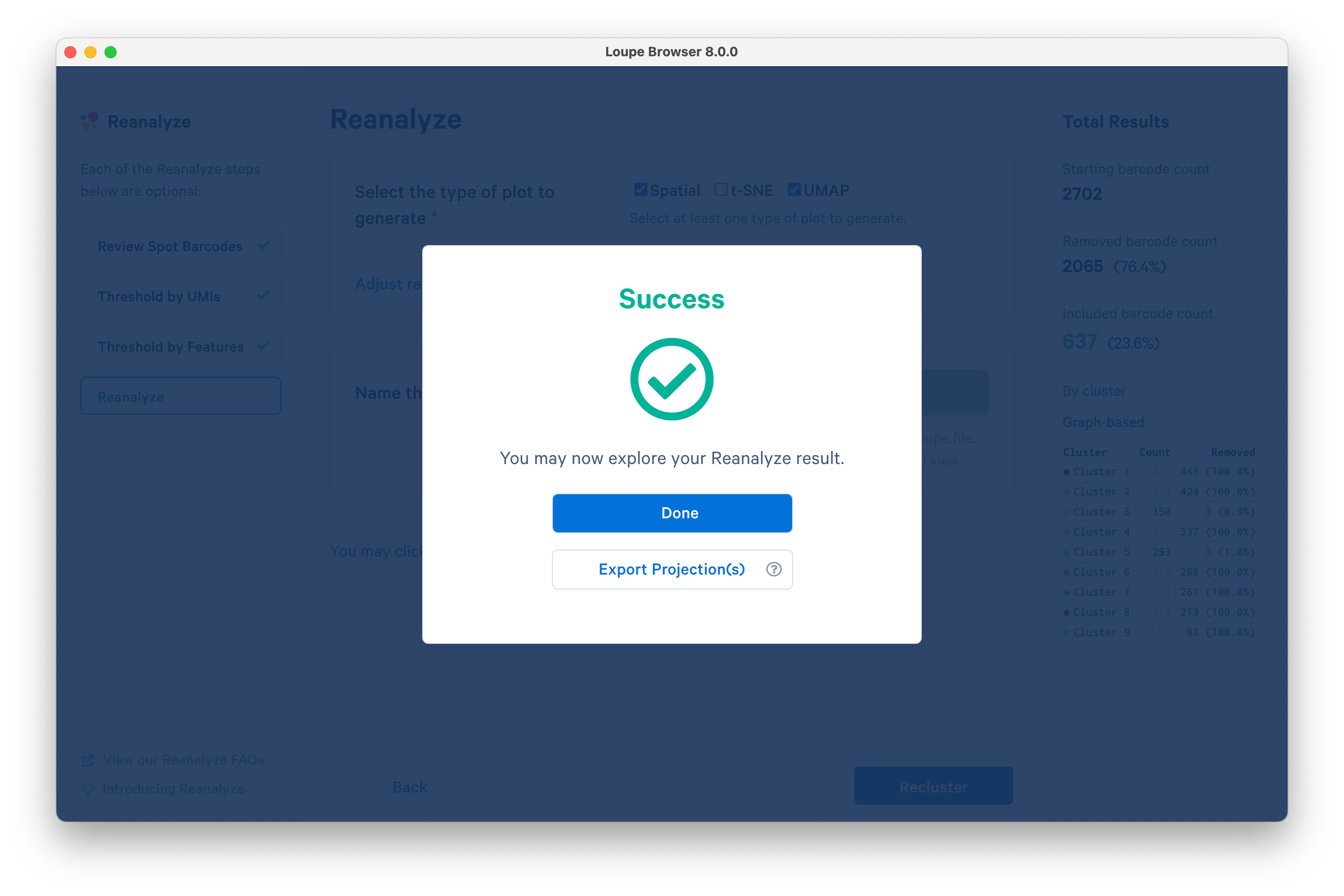
Selecting Done will close the recluster window, and update the primary Loupe window to the new projection and category.
Alternatively, export the projection coordinates of the spatial plot, t-SNE and/or UMAP projection(s) for the reclustered data by clicking Export Projection(s). Selecting this option will follow the same steps as above in addition to downloading a .zip file to a local directory of your choice.
In the primary Loupe window, the reclustered plots appear beneath the pipeline-generated groups in the Clusters view.
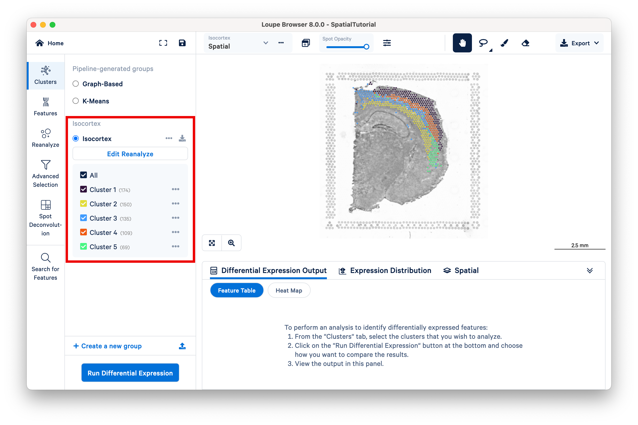
Multiple reclustered datasets can exist within the same Loupe file, with each listed under the unique name provided in the reclustering window.
All Loupe functions applicable to the full dataset are also applicable to the reclustered dataset, albeit restricted to only a subset of the spots from the original dataset. Users can open multiple linked windows, evaluate significant genes, and explore active features. Users can also visualize projections from reclustered datasets independently as well as projected onto the original dataset space.
Saving the .cloupe with the reclustered dataset will save the reclustered projections and categories. Finally, it is possible to adjust the reclustering or recall its parameters by clicking on Edit Reanalyze.
In this section, we covered how to use Loupe's Reanalyze feature to review spot barcodes, threshold by UMIs or features, and export projections.
In the final section of this tutorial series, you will learn how to share results with a colleague.