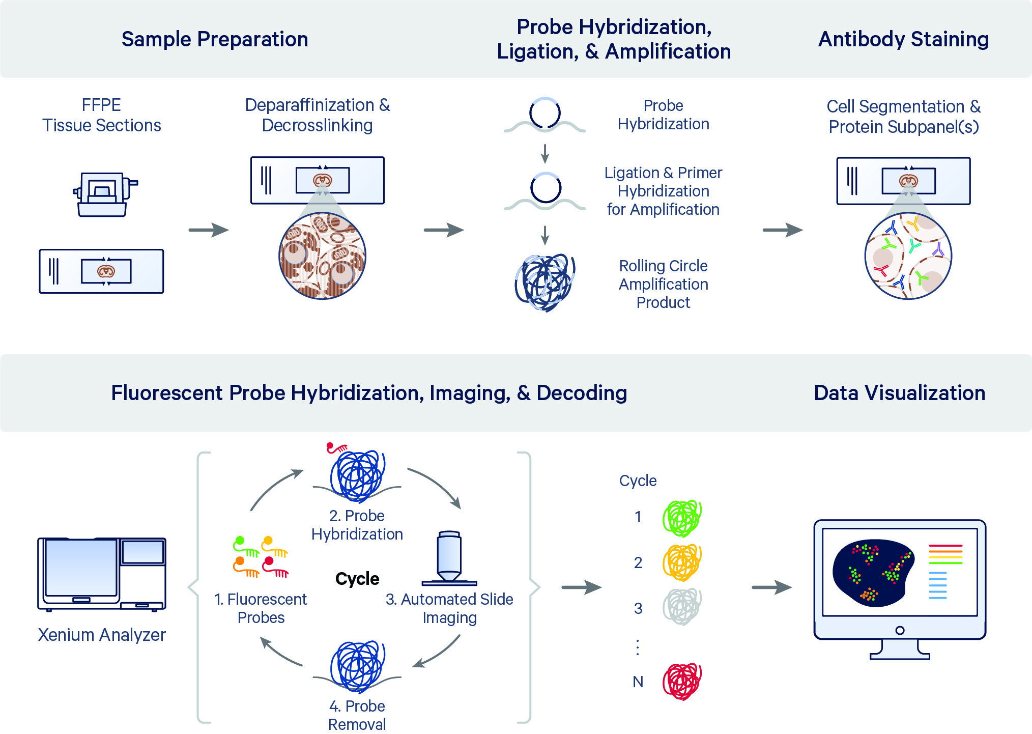
The Xenium In Situ Gene and Protein Expression with Cell Segmentation Staining assay (CG000819) assays RNA and protein at the subcellular level in human formalin fixed & paraffin embedded (FFPE) tissue sections (referred to as Xenium Protein assay hereafter). The data acquisition steps and algorithms for processing transcript data to generate Xenium Onboard Analysis (XOA) outputs are described on the main Algorithm Overview page.
On this page, we describe the data acquisition steps and algorithms for processing protein data to generate XOA outputs. Like the RNA images, the internal image sensor captures data across multiple Z-planes for protein images with a 0.75 µm step size across the entire tissue thickness for every field of view (FOV) in the user-selected region (see Region Selection Guidelines in the Xenium Analyzer instrument user guide). Image data are captured for multiple fluorescence channels in every cycle, which are processed and stitched to build a spatial map of the protein expression across the selected tissue section.
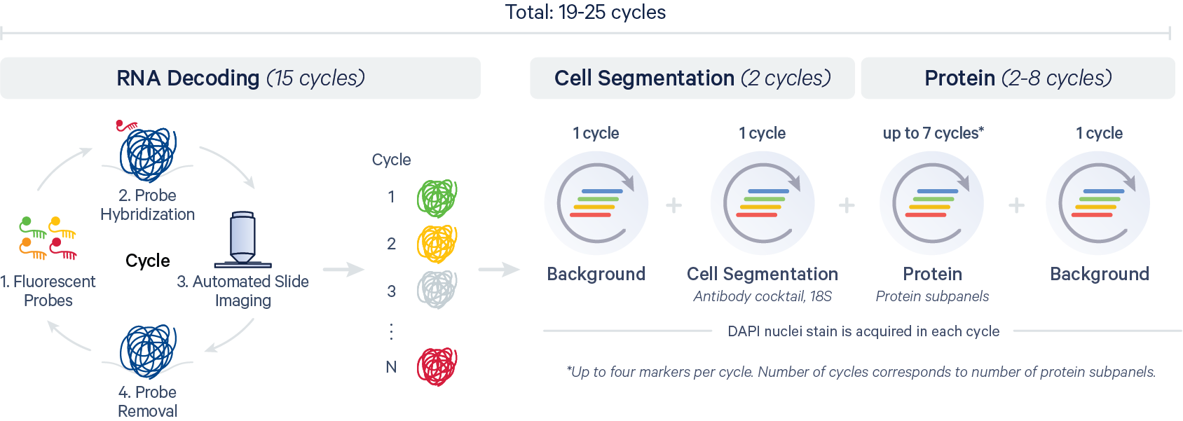
After the RNA decoding and cell segmentation cycles, the Xenium Protein assay includes up to seven additional cycles to image protein subpanel markers. A second background image is acquired for performing background subtraction on the protein image data.
The XOA v4.0 pipeline introduces support for analysis of protein data. The high-level pipeline steps for the Xenium In Situ Gene and Protein Expression with Cell Segmentation Staining assay (CG000819) are shown in the diagram below:
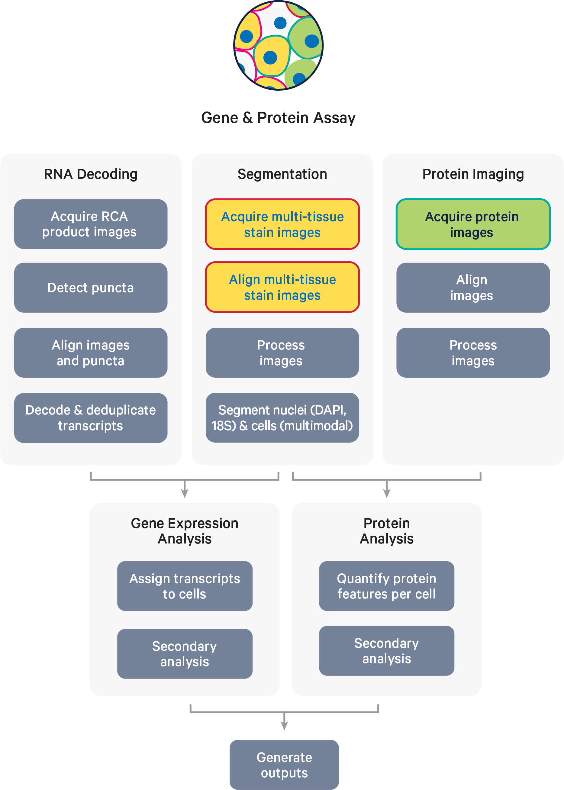
The following steps are the same as those described for gene expression only datasets (see main Algorithm Overview page): image processing (DAPI, cell segmentation images), nucleus and cell segmentation, RCA product image registration, decoding, deduplication, and gene expression secondary analysis.
XOA v4.0 introduces algorithms to process protein data. The protein image processing, mean intensity, and secondary analysis algorithms are described in the sections below.
The protein image process algorithms produce a 2D projection for each image stain (output in the morphology_focus/ directory).
The DAPI images from these protein cycles are aligned to the cycle 1 DAPI image, so they are in the same coordinate system. Protein images are sampled based on a global focus map, derived from the DAPI, background, and cell segmentation stain Z-stacks. A deconvolution algorithm is then applied and the middle slice of the deconvolved image volume is selected for both background and protein cycles. Image features will appear sharper and fluorescence intensity values lower as a result of image deconvolution algorithm improvements. These are the same steps described for DAPI and cell segmentation images here.
Next, the 1st and 2nd background cycle images are used to estimate background, which is subtracted from each deconvolved protein image to help offset the effects of autofluorescence. The estimated background image is locally adjusted for uneven brightness patterns by scaling the background in 32 x 32 pixel patches to create a subtracted image with uniform background intensity.
During background subtraction, there may be cases where the background image pixel is brighter than the protein image pixel, resulting in negative values. However, downstream analysis tools may not be able to read signed integer data. To maintain compatibility with other analysis tools and preserve the information that would have been lost in protein images due to clipping negative values to zero, XOA v4.0 instead adds a fixed offset value of 100 units to each pixel. This offset is not applied to cell segmentation images.
An example is shown below. For simplicity, we illustrate pixel values for one protein marker in a 3 x 3 pixel "cell" with an offset of 100 units. The yellow pixel's negative intensity value is retained by applying the offset, instead of clipping it to zero.
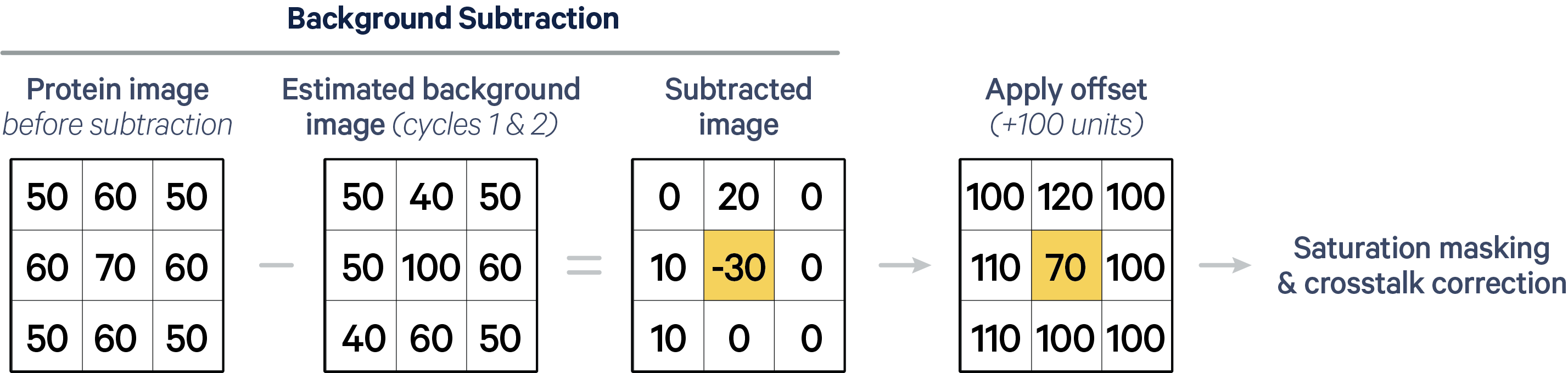
For guidance on accounting for this offset value in outputs, read the section below.
Protein images then undergo a masking step using saturation QC mask images (output in morphology_focus_qc_masks/).
- Adjust for exposure time differences: In the image processing pipeline, XOA uses the background images to determine which pixels to mask. Since each protein image is captured with different exposure times compared to the background images, the intensities of the background images are adjusted accordingly.
- Create QC masks for each protein image: We identify pixels in the adjusted background images used for subtraction and/or of a different acquisition channel that were saturated. This step is critical because the crosstalk correction algorithm requires valid pixels across all channels for a given cycle. In the binary morphology focus QC mask, pixels have two possible values: saturated pixels = 255 (white) and unsaturated pixels = 0 (black).
- Use QC masks to mask protein images: Pixels with saturated autofluorescence are masked in the protein images (set to zero) because they violate the assumptions of the background subtraction and crosstalk correction algorithms. In some cases, when comparing protein and QC saturation masks, you may notice some zero pixel values in protein images are non-zero due to JPEG2000 image compression. Saturated protein image pixels are not masked in order to retain potential positive protein signal.
Finally, a spectral crosstalk correction is applied to remove signal bleedthrough from other channels for protein images. Different spectral channels can interfere with each other. This step corrects that bleedthrough by removing the predicted contribution of each of the fluorophores from channels that are not intended to detect them.
These processed images are provided in the Xenium Onboard Analysis output bundle as multi-file OME-TIFF files, one per channel, in the morphology_focus/ directory. Outputs are detailed here.
The Xenium software suite automatically accounts for the offset applied after background subtraction in the protein data outputs and when visualizing the protein images.
The cell-feature matrix files contain protein expression information quantified by a per-cell mean fluorescence intensity statistic. In each cell, every protein marker feature is quantified by calculating the mean fluorescence intensity using pixels in the 2D cell segmentation mask.
- This statistic does not include intensity values measured outside cell boundaries and it is not a count value.
- XOA automatically excludes pixels that do not yield reliable protein signal. These invalid pixels stem from: 1) saturation in the scaled background image (recorded in the saturation QC mask), or 2) production of non-existent pixel regions from image distortion correction or stitching at tissue ROI edges (recorded as 0s or 1s in morphology focus image). The presence of invalid pixels primarily affects reanalysis of protein image data. Xenium Ranger also excludes invalid pixels, but if you recalculate protein mean intensity in third-party tools, we recommend applying the same filtering criteria or limiting analysis to regions with valid pixels to avoid artifacts that can occur at ROI edges.
Here is an example for calculating the scaled mean fluorescence intensity for one protein in the 3 x 3 "cell" example illustrated above:
- Total cell area: 3 x 3 = 9 pixels
- For simplicity, we assume no further changes to the pixel values during crosstalk correction in this example. Total fluorescence intensity per cell per protein: 100 + 120 + 100 + 110 + 70 + 100 + 110 + 100 + 100 = 910 units
- Mean intensity is calculated as the total fluorescence intensity per cell per protein divided by the total cell area in pixels. Protein mean intensity for this "cell": 910 / 9 = 101.11
- XOA subtracts the 100 unit offset prior to saving the values in the cell-feature matrix: 101.11 - 100 = 1.11
- The mean fluorescence intensity is then scaled by multiplying the average pixel values by a scaling factor of 10 and rounded to an integer value in XOA v4.0. The scaling factor is applied to retain precision, as the matrix format only supports integer values. The scaling factor is stored in the cell-feature matrix HDF5 file. Multiply by scaling factor of 10 and round to integer value: 1.11 x 10 = 11.1 -> round to 11
- The final scaled mean protein intensity value for this example "cell" is 11.
These values are rescaled as mean fluorescence intensity (divided by 10) for the following outputs to use the same scale as the protein image pixel intensities:
- In the analysis summary (per-cell; Protein Analysis tab)
- Xenium Explorer v4.0 (per-cell or per-selection; Selected ROIs)
Xenium Explorer v4.0 automatically subtracts the offset from the intensity slider display range when you visualize protein images. This keeps the image values consistent with per cell and per selection quantification stats, which are read from the cell-feature matrix.
Xenium Ranger v4.0 follows the same algorithms as XOA v4.0 and subtracts the offset to recalculate mean fluorescence intensities if cell segmentation is changed.
--transcript-assignment) of a Xenium Protein dataset, the requantification and reanalysis of protein data will be disabled because there are no cell masks for calculating mean fluorescence intensity (described on Xenium Ranger algorithms page). The cell-feature matrix will only contain the updated gene expression counts based on the imported segmentation results.Community-developed tools are not necessarily set up to automatically account for this offset value. For downstream analysis workflows, here are a few scenarios for deciding whether you need to manually account for the offset:
| Analysis | Workflow example | Manually subtract offset? |
|---|---|---|
| Gating cells just with the cell-feature matrix data | For example, using Python to plot histograms of the scaled mean protein intensities from the matrix. Since the offset is already subtracted from the matrix values, no further changes are needed. | No changes needed |
| Gating cells starting from the protein image data | For example, using QuPath to do cell segmentation, quantification, and gating. The distribution will be shifted by 100, but no need to worry about the offset while working in QuPath. If you import the QuPath cell segmentation to Xenium Ranger to integrate protein and RNA data, then Xenium Ranger will subtract the offset. | No changes needed |
| Picking thresholds using the protein image data and then filtering cell-feature matrix by protein quantity | For example, importing XOA cell segmentation results into QuPath to see histograms and manually set thresholds, and subsequently using those thresholds to filter the cell-feature matrix by scaled mean protein intensities. | Yes, you need to subtract 100 from the thresholds |
For protein secondary PCA, UMAP, clustering, differential gene express analysis, XOA processes the protein-only features with the same filtering and secondary analysis algorithms as for RNA (described here).
The pipeline also produces outputs quantifying the protein features that exhibit higher expression levels within a specific cluster compared to the rest of the sample (for each clustering method). The per-cell protein mean fluorescence intensities are standardized using a Z-score normalization process, which enables comparison of proteins with different distributions. For each protein feature, the median Z-score is computed across the cells within each cluster. The calculation is shown below:
For each protein feature and each cluster i, we compute the median Z-score of all its cells, based on the average and standard deviation of that protein feature’s expression in the rest of the clusters.
Where
- identifies a protein feature;
- is the index of a cell in the -th cluster;
- is the average Z-score of the -th cluster for the protein feature ;
- is the number of cells in the -th cluster;
- is the expression of protein feature for the -th cell the -th cluster;
- and and are respectively the median and the standard deviation of the expression of protein feature across all cells that are not in the -th cluster.