Loupe v8.0 and Space Ranger v3.0 now support Visium HD Spatial Gene Expression (“Visium HD”) to achieve single cell-scale resolution. Each Visium HD slide features more than 11 million 2 x 2 µm squares, each embedded with a unique barcode, within a 6.5 x 6.5 mm capture area. In this tutorial, we demonstrate a human colorectal cancer (CRC) dataset to illustrate the potential of Visium HD to improve our understanding of the biology of this heterogeneous disease.
Colorectal cancer (CRC) is the second leading cause of cancer related deaths globally, accounting for 9.4% of cancer-related deaths (0.9 million) in 2020, a number that is predicted to double by 2035 (Xi & Xu 2021, Hossain et al. 2022). Although researchers have learned much about the transcriptional profiles of these tumors through single cell profiling (reviewed by Wen et al. 2023), the intricacies of the tumor microenvironment remain poorly understood. In particular, there is much to be learned about the local interactions of immune and non-immune cells in the tumor microenvironment of CRC.
In this tutorial you will learn how to:
- Explore a Visium HD dataset with the updated Loupe Browser 8.0 user interface
- Review unsupervised clustering results
- Use goblet cell markers and the microscope image to visually assess transcript localization
- Map marker genes for tumor cells, cancer-associated fibroblasts, macrophages, and neutrophils to get a closer look at the tumor microenvironment
- Create a new group using known marker genes and perform differential gene expression to discover new markers
- Plot co-expression of tumor and fibroblast genes
Once you have downloaded and installed Loupe Browser v8.0, you can find the Visium HD colorectal cancer tutorial on the landing page, under Tutorial files.
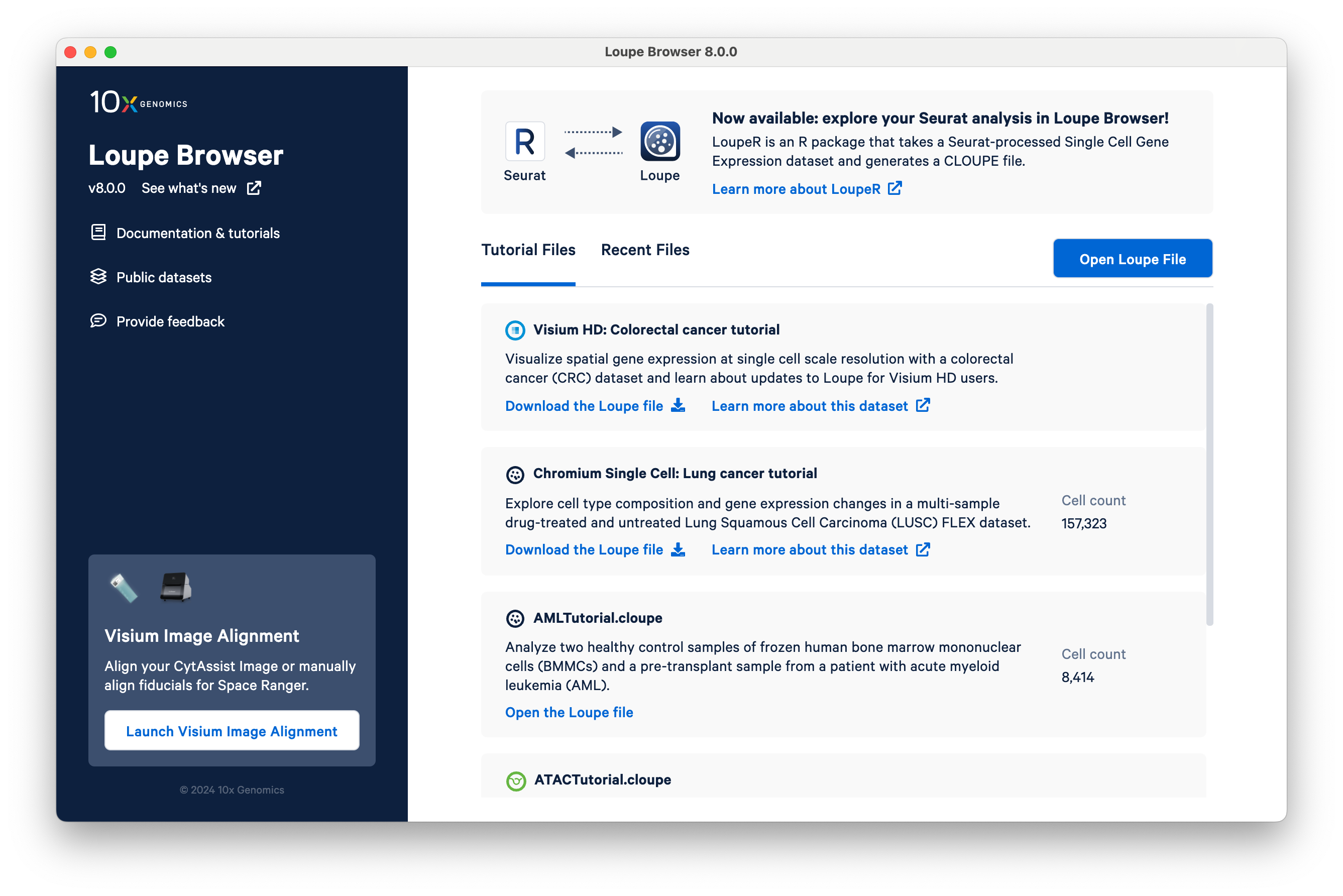
Click Download the Loupe file. The file is 7.7 GB. Then open the cloupe_008um.cloupe file. The file name matches what is output from Space Ranger by default (8 µm bin size). Here, we rename it to CRC_008um.cloupe.
After loading the dataset, take a minute to orient yourself. If you have used Loupe recently for other 10x datasets, the user interface should be familiar. The same tools used for other spatial and single cell datasets are still applicable to Visium HD.
If you are a new Loupe user, it may be helpful to review the Loupe Spatial Navigation tutorial for a comprehensive walkthrough of all the features. Here, we analyze Visium HD data, no previous experience required.
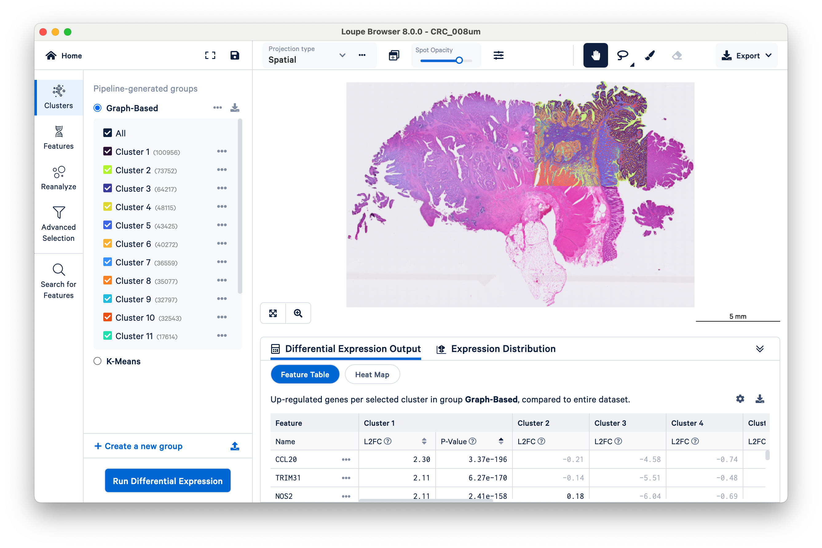
The microscope image (in this case, a brightfield H&E image) and HD gene expression data are visualized together in the center of the screen. Notice that the scale bar is set to 5 mm to start. The scale bar will change as you zoom in and out. Also observe the location of the 6.5 x 6.5 mm capture area, where the gene expression data are, relative to the overall tissue image.
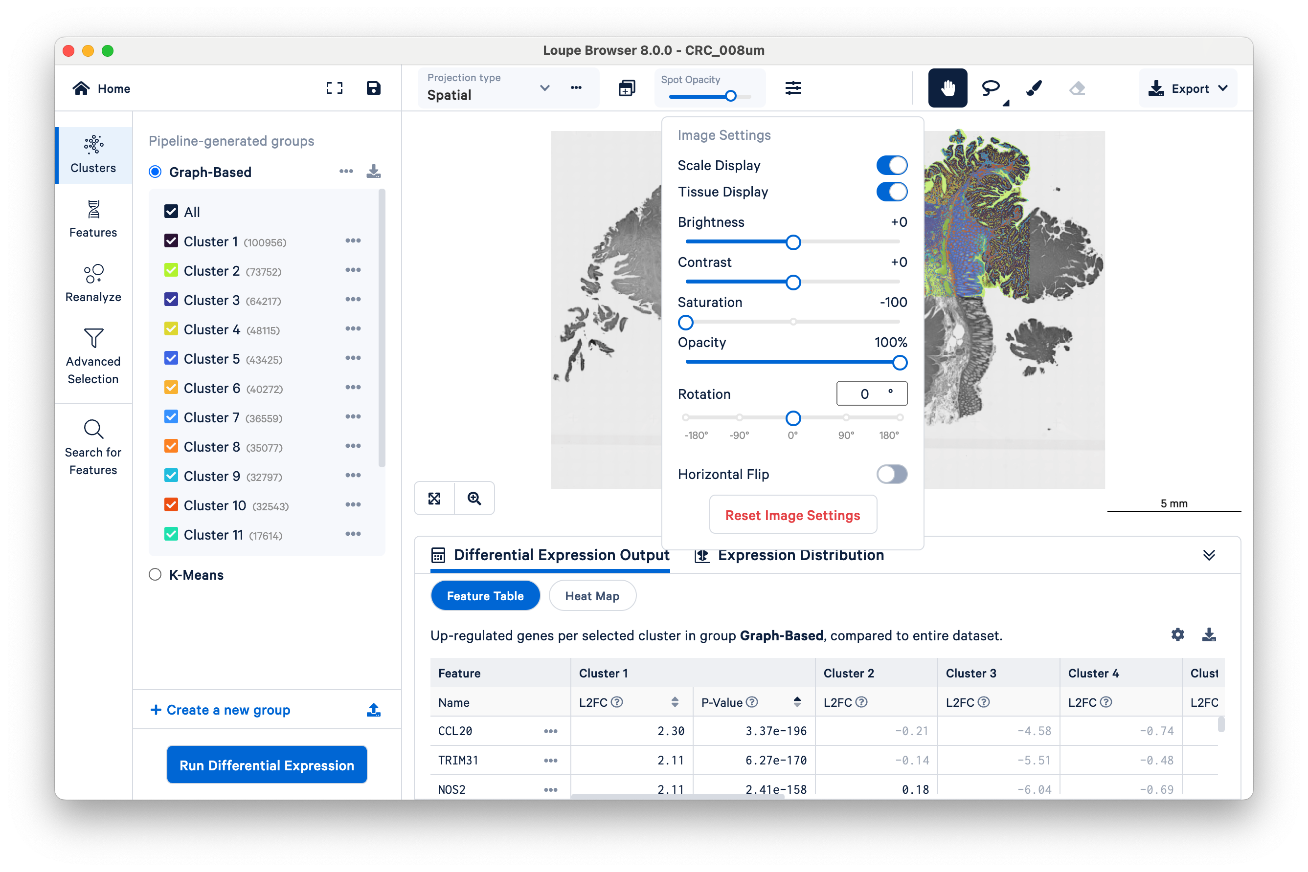
This becomes more obvious if you reduce the saturation of the microscope image with the slider under the projection settings:
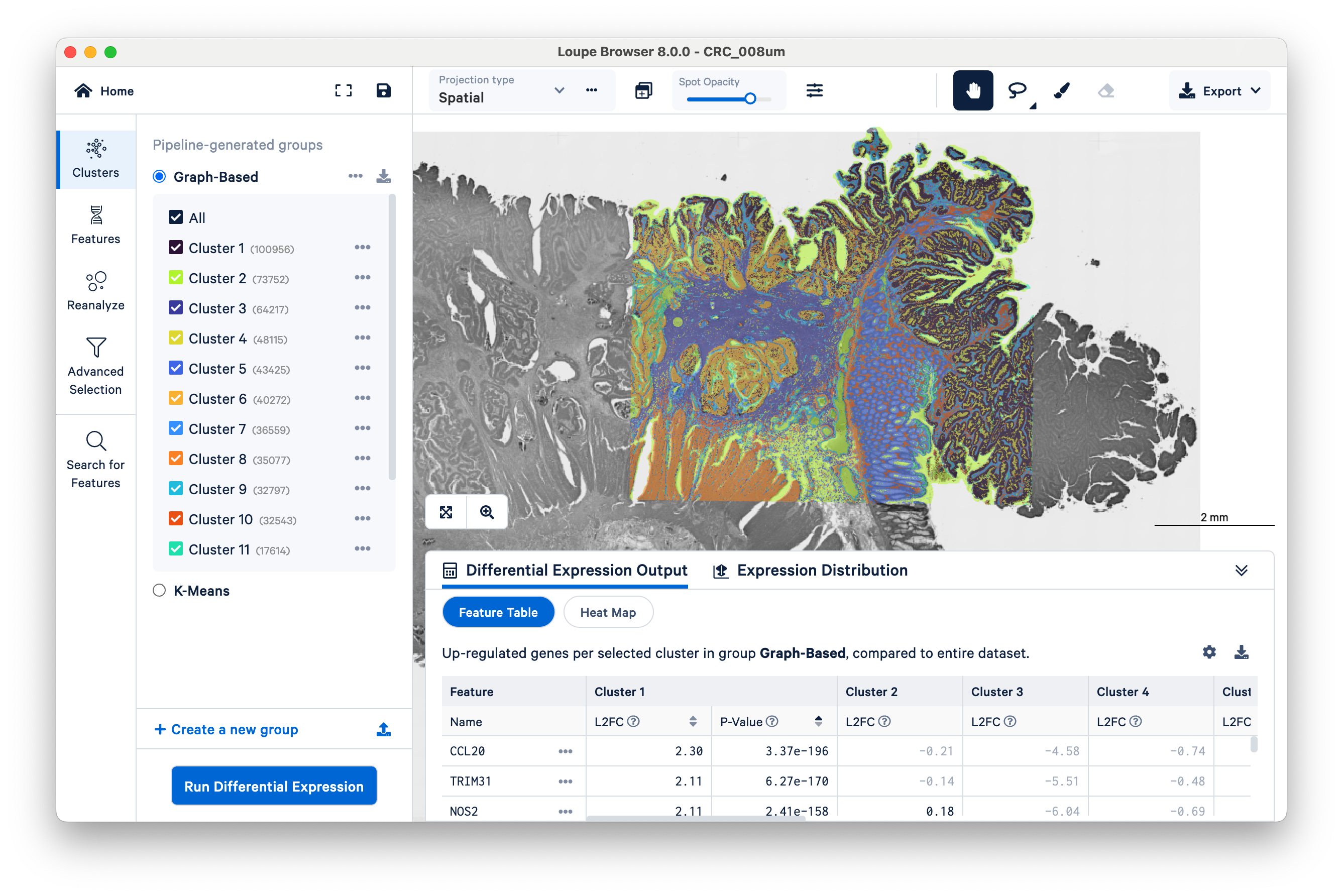
Then zoom in a bit to fill the frame with the capture area:
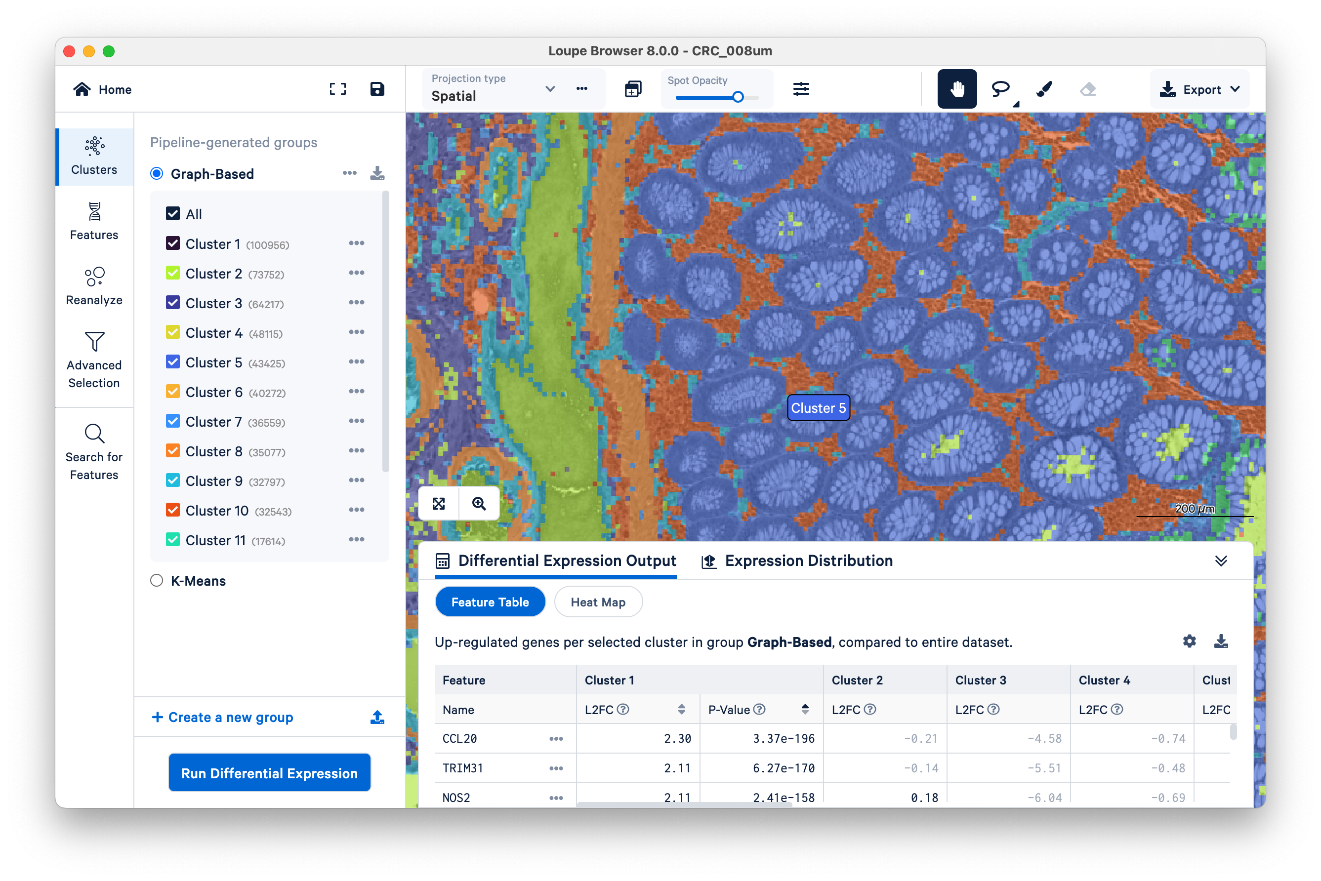
By default, Loupe displays graph-based clustering results. You can also toggle to K-means clustering, which requires you to choose a K value (the number of clusters) ranging from 2 to 10. Both graph-based and K-means are different varieties of unsupervised clustering, meaning that the algorithms find structure in the gene expression data on their own, without input labels or spatial information. As you toggle among the different pipeline-generated groups, notice that the colors displayed on the center image will match those in the Clusters panel.
In this particular dataset, Space Ranger defined 15 graph-based clusters. The exact number of graph-based clusters produced is dependent on the algorithm and will vary among datasets.
We will let the whole transcriptome data help us annotate which clusters, if any, correspond to tumor tissue, cancer-associated fibroblasts, and other tumor microenvironment structures. But first, let’s start with a cluster that matches tissue morphology very closely.
Zoom in a bit more and mouse over the circular structures (cluster 5). Observe that the cluster name changes as your mouse moves over the image:
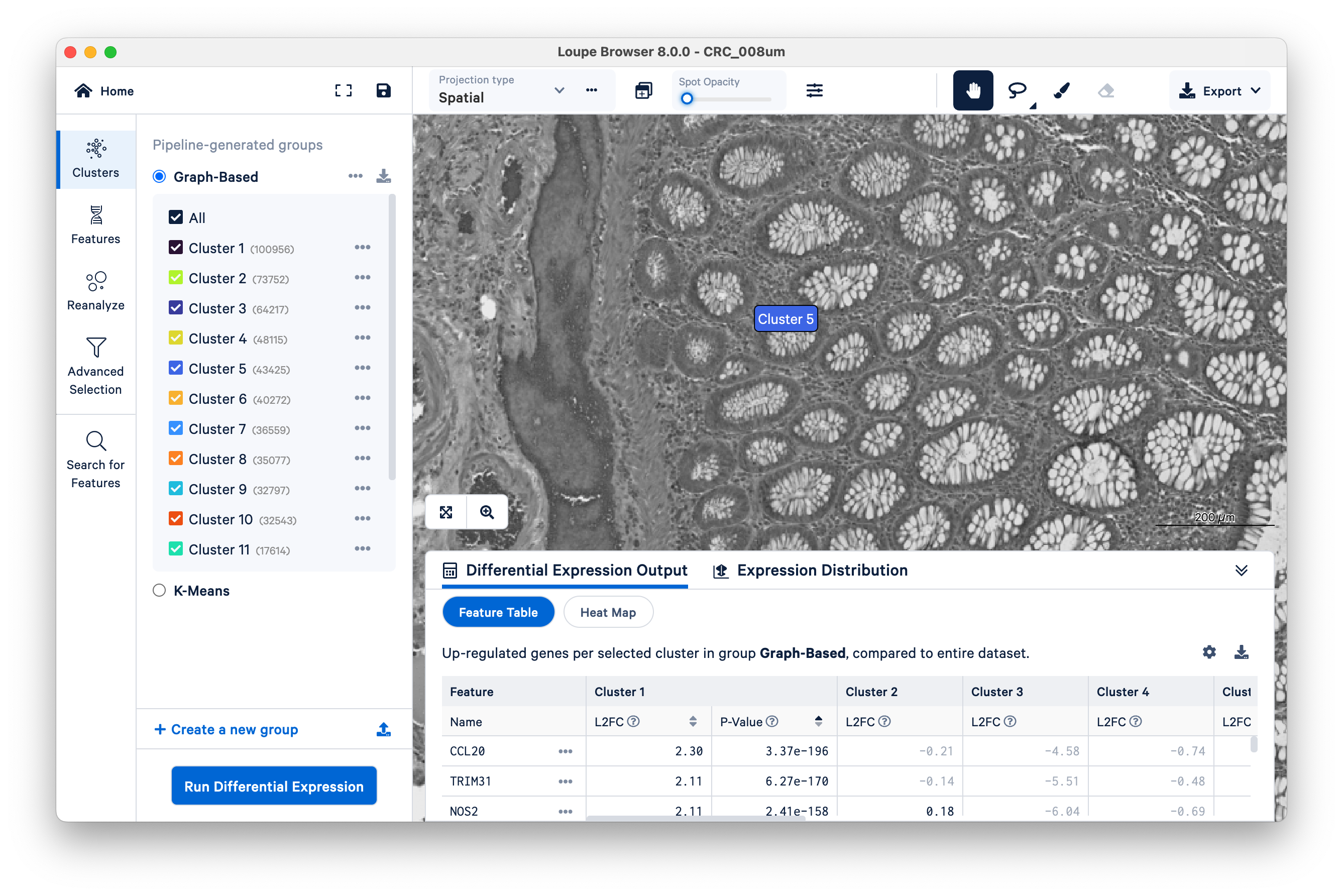
Toggle the Spot Opacity to zero to see the underlying tissue image without the colors. Even with the colors off, you can still mouse over the image and see where Cluster 5 is.
Now slide the opacity back up, and unselect all clusters except Cluster 5.
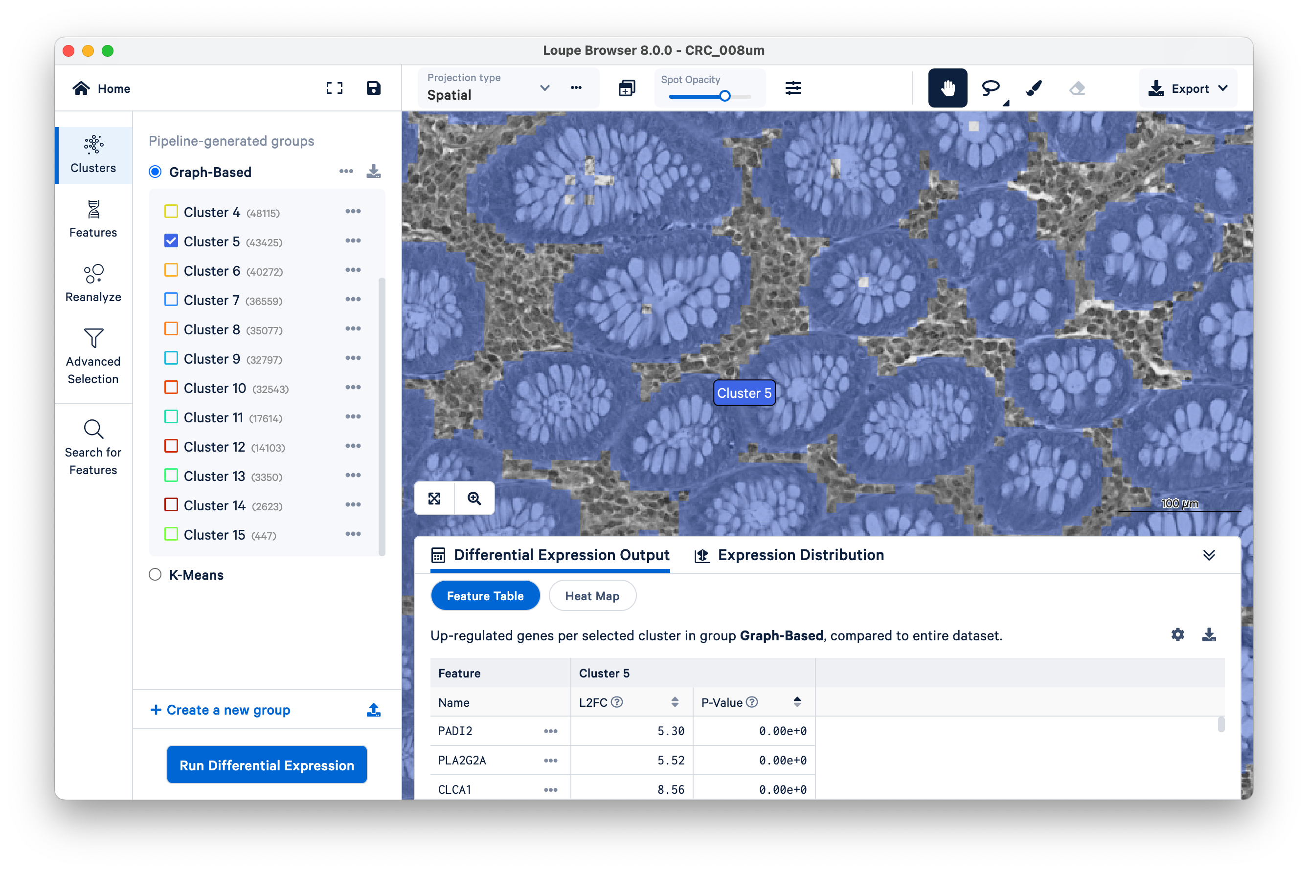
In this case, Cluster 5 corresponds very closely with glands of normal colon mucosal tissue, composed mostly of goblet cells and normal mucosal cells. Next, we will use these structures to assess transcript localization using known marker genes.
Here, we illustrate how you can use Loupe Browser to assess the specificity of marker genes to their expected locations in the tissue. Start by clicking on Features on the left-hand side.
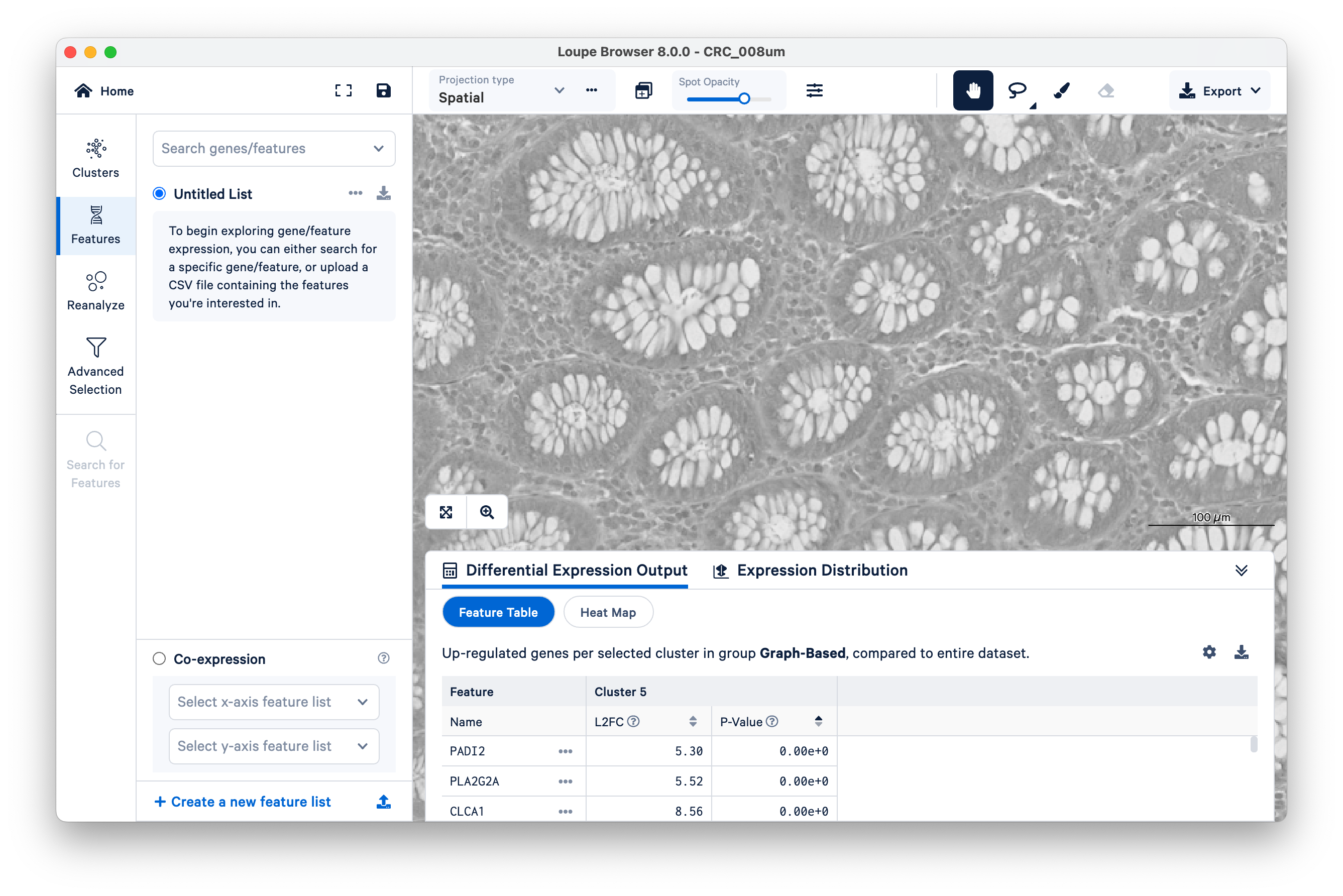
We will use FCGBP and MUC2 as marker genes for goblet cells, which we only expect to show up in the glands of normal colon mucosal tissue. Type in the gene names in Search genes/features to add them to your Untitled List. Then choose Combine all below and zoom out a bit.
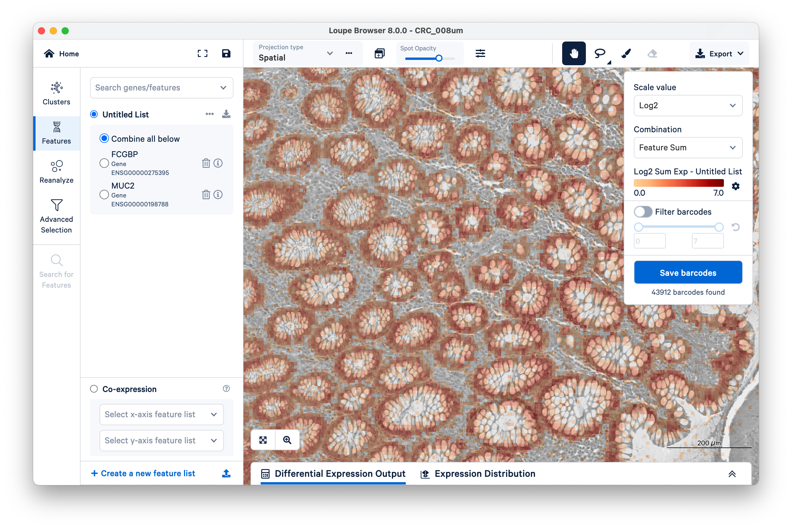
You can see that for the most part, these genes are being expressed where they are expected. But a few transcripts are scattered elsewhere. These could be potentially mislocalized transcripts, barcode correction errors, or barcode synthesis errors.
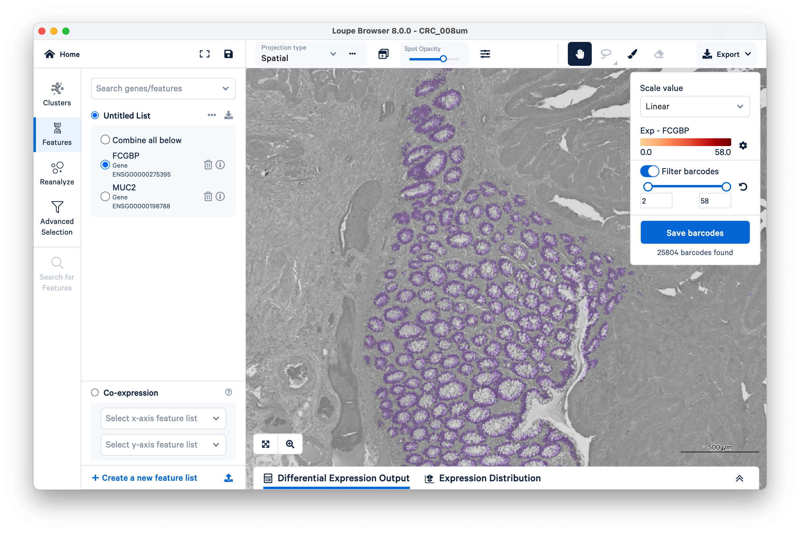
To quantify these, start by selecting FCGBP. Then change the scale value from Log2 to Linear.
This will show UMI counts directly (on a linear scale instead of log-transformed).
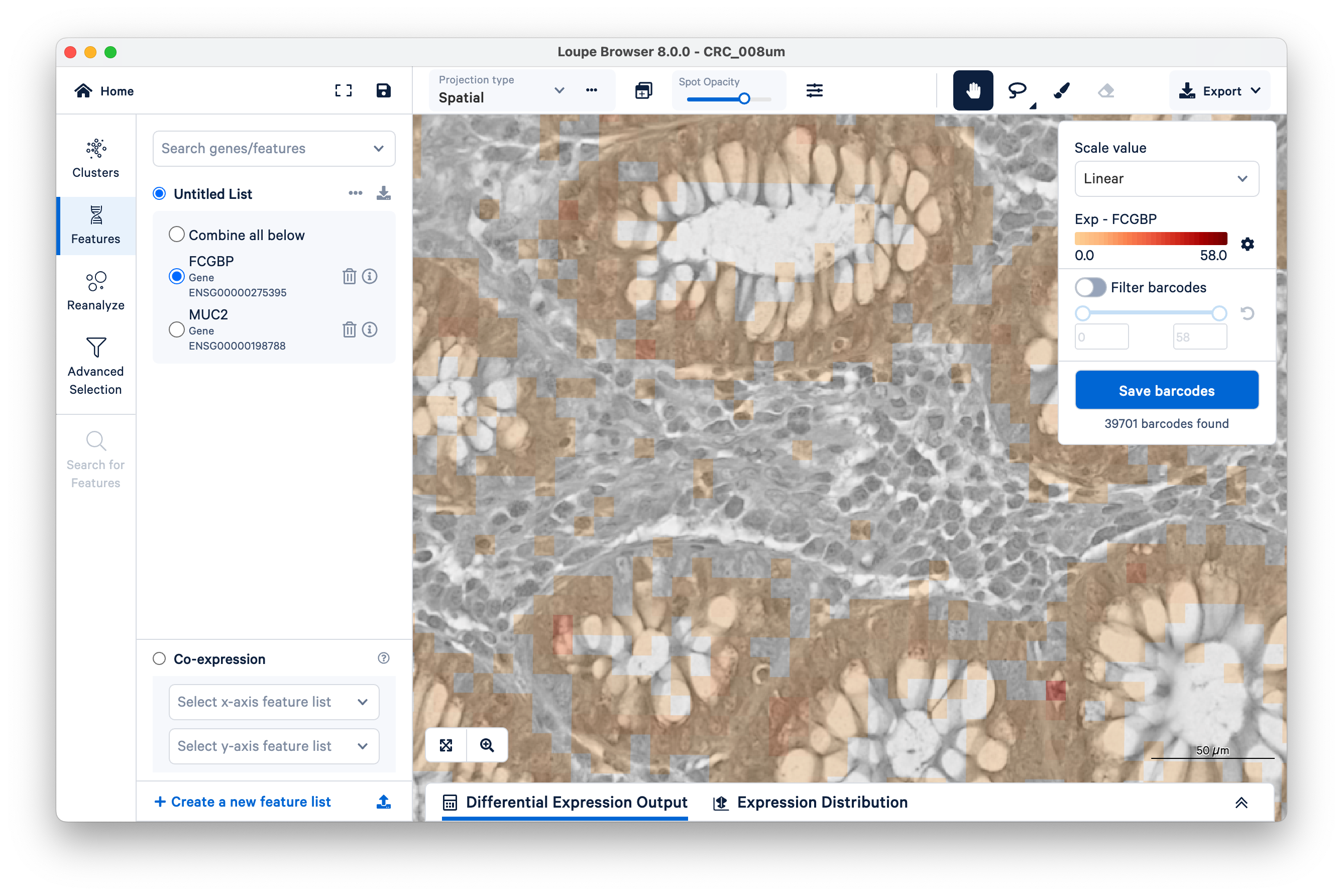
Observe the squares scattered between the glands. These are 8 x 8 µm bins, each composed of 16 barcoded squares (2 x 2 µm). You can zoom in and use the scale bar to confirm.
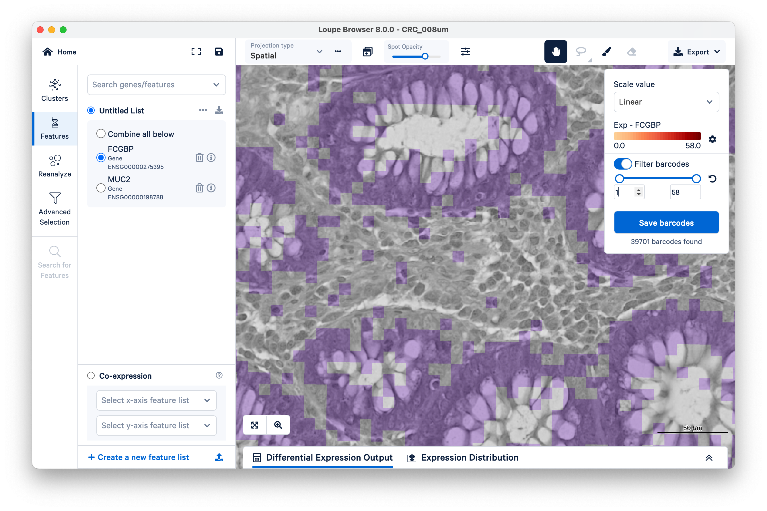
Next, on the top right, switch on Filter barcodes and set the minimum to 1.
Now shown in purple are all bins that have between one and 58 UMIs. (In this case, 58 is the maximum UMIs observed per bin in this dataset). Notice there are still those same squares lighting up between the glands.
Now increase the lower limit to two UMIs. Observe that most of the intervening bins disappeared.
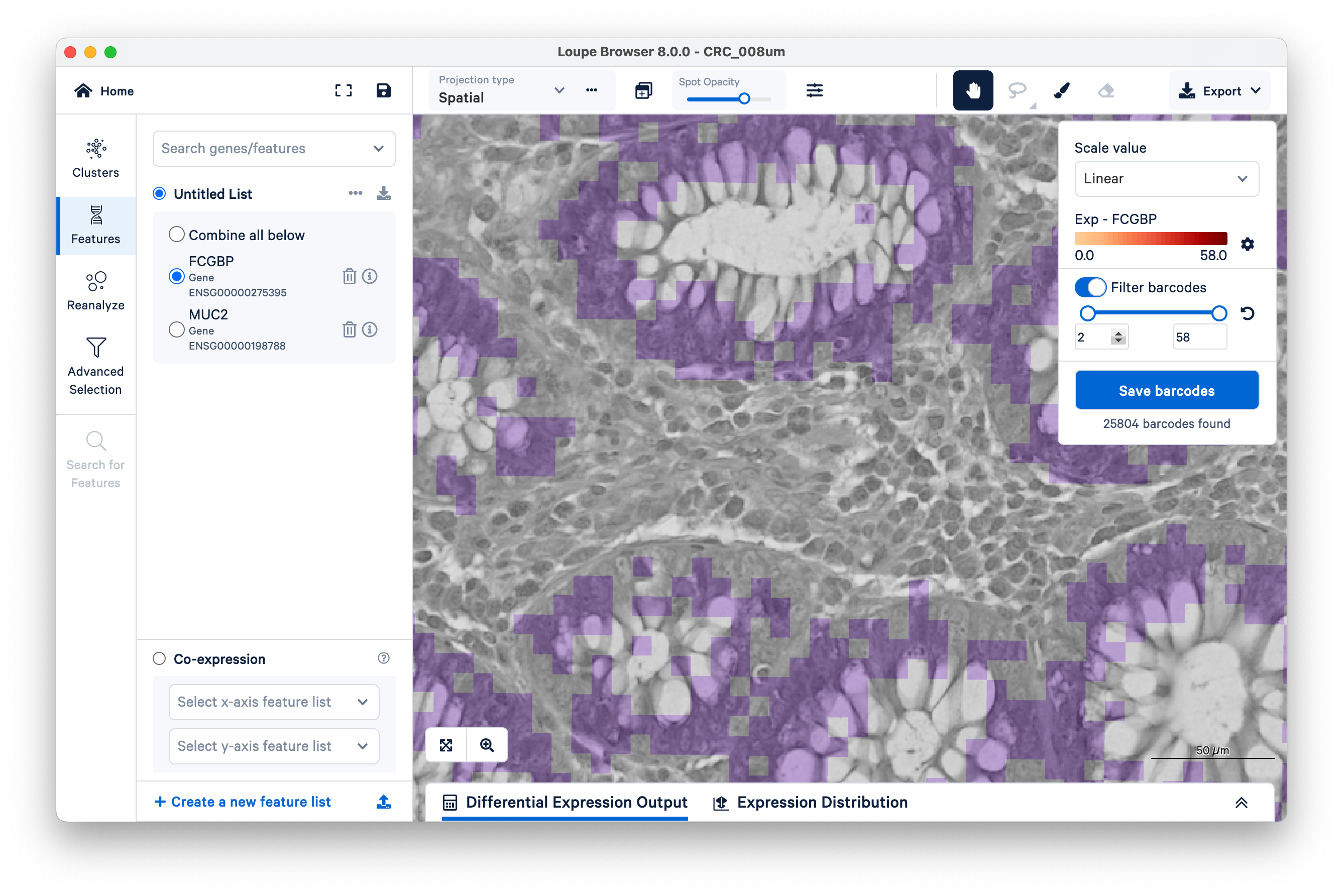
Zooming out, we can clearly see that setting a minimum as low as two UMIs per bin for the FCGBP gene is enough to filter out nearly all mislocalized transcripts and cleanly delimit the goblet cells. You can achieve similar results with MUC2.
You can save your bins as a new group or cluster for downstream analysis. We will do this shortly with tumor markers. For now, let us continue to map specific cell populations.
Visium HD has single cell-scale resolution, meaning that the bin size of 8 µm is smaller than most mammalian cells, but any given bin can still include a mixture of cell types. So although bins don’t correspond 1:1 to cells in the same way as barcodes do in single cell assays, we can still map the locations of specific cell populations at high resolution using marker genes – but we can’t guarantee those bins don’t also contain other cell types as well.
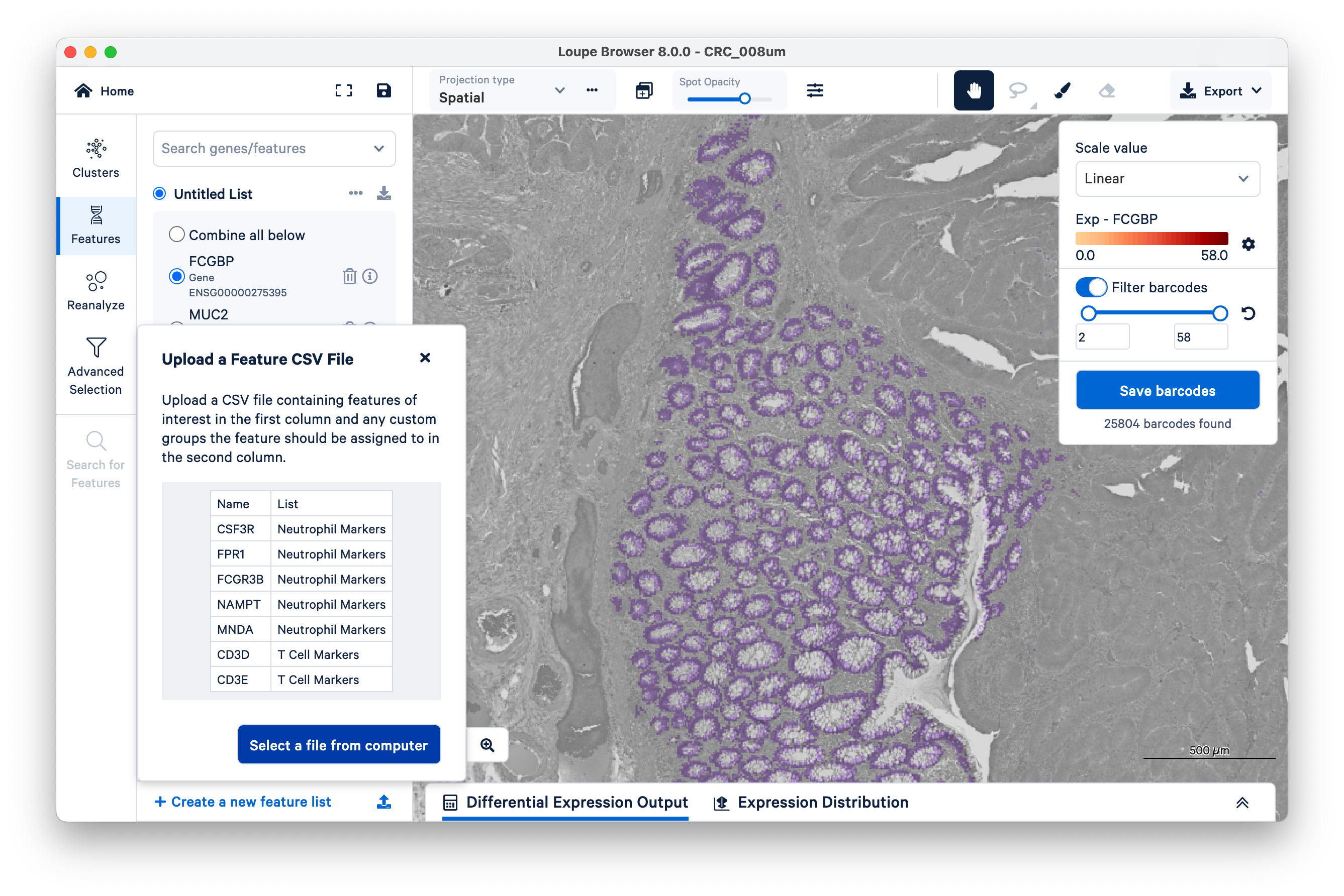
Searching for genes one at a time can be slow if you have many genes. To save time, you can import and export your gene lists as CSV files.
To continue, download the following CSV files for different tumor microenvironment cell markers.
To import the CSV files, click the upload icon on the bottom left of the screen. Then select a file from your computer to upload one list at a time.
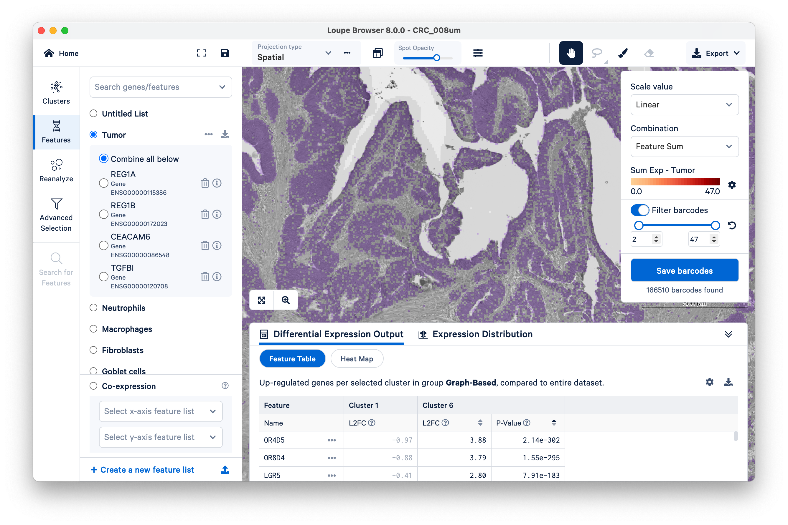
First, look at where the tumor markers are being expressed. These include REG1A, REG1B, CEACAM6, and TGFBI.
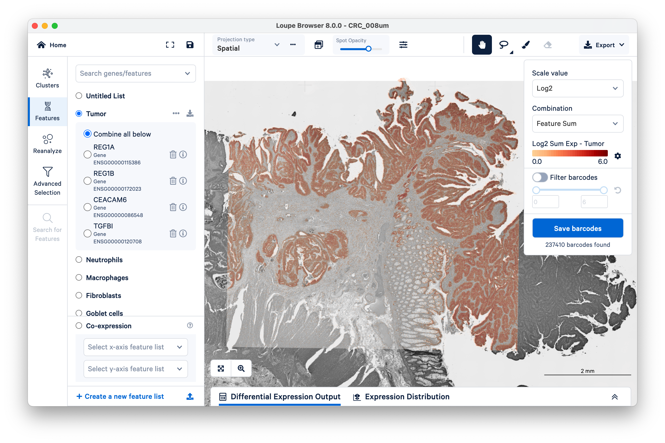
You can use these markers to figure out which graph-based cluster corresponds to tumor tissue. Zoom in a bit to get a closer look (with the scale bar set around 500 µm).
Then switch back to Clusters on the left-hand side. Mousing over the same tissue, and toggling back and forth between Clusters and Features a couple of times, we can see that clusters 1 and 6 approximately match the tumor tissue.
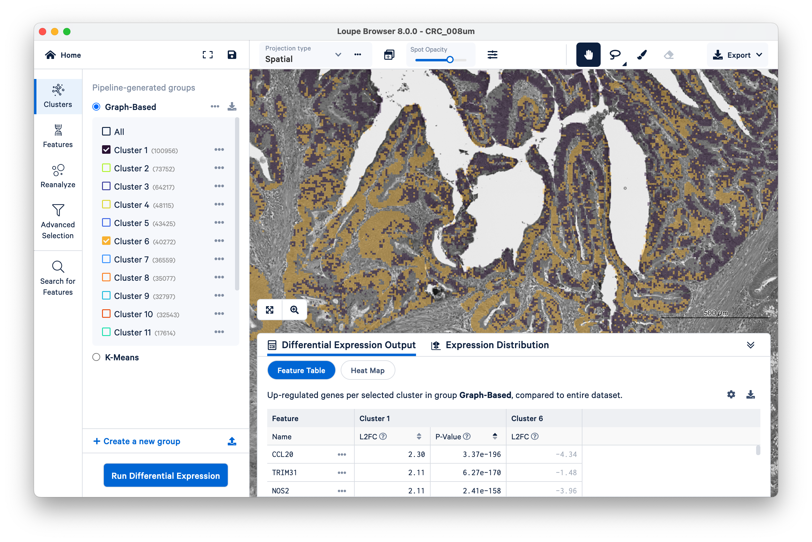
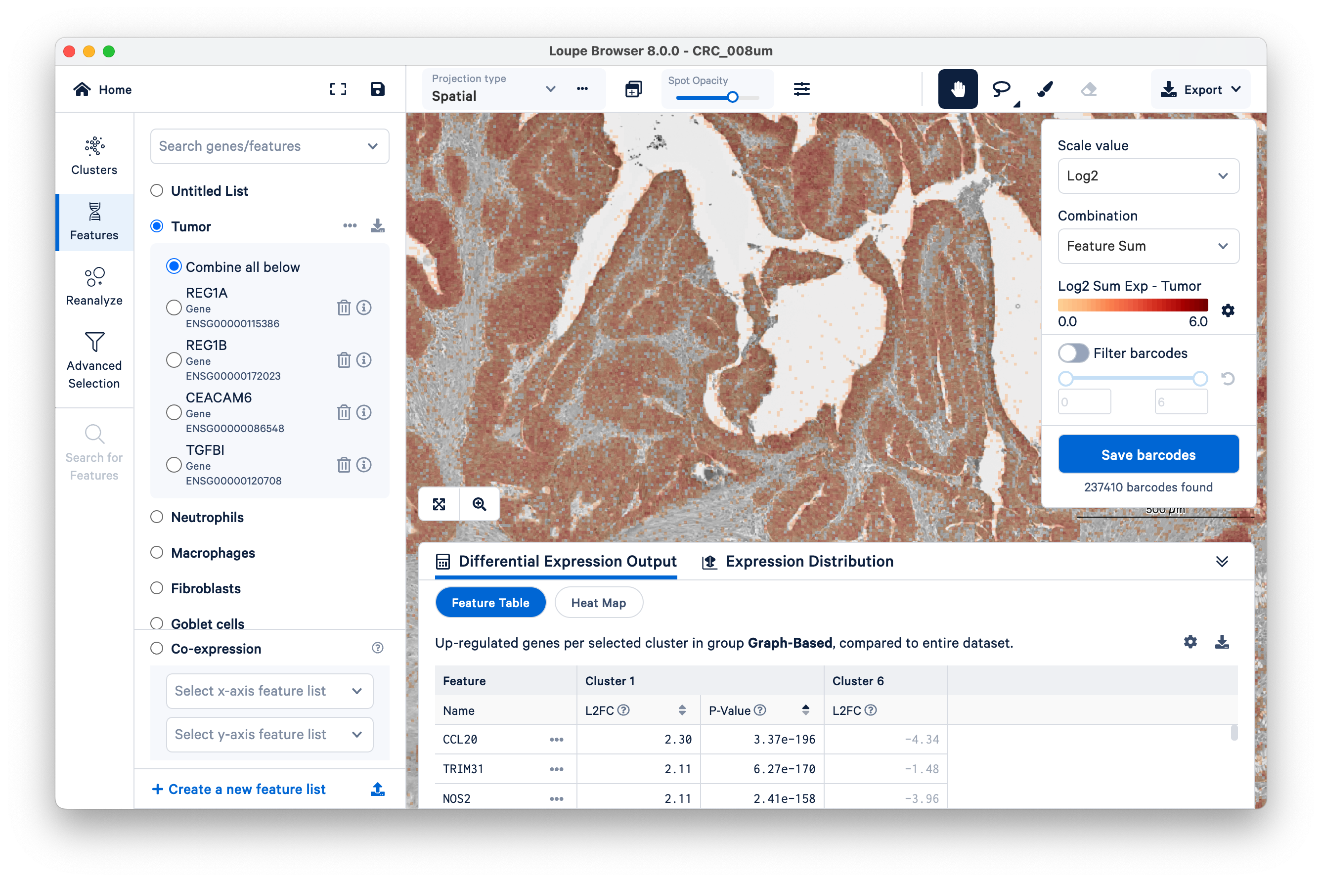
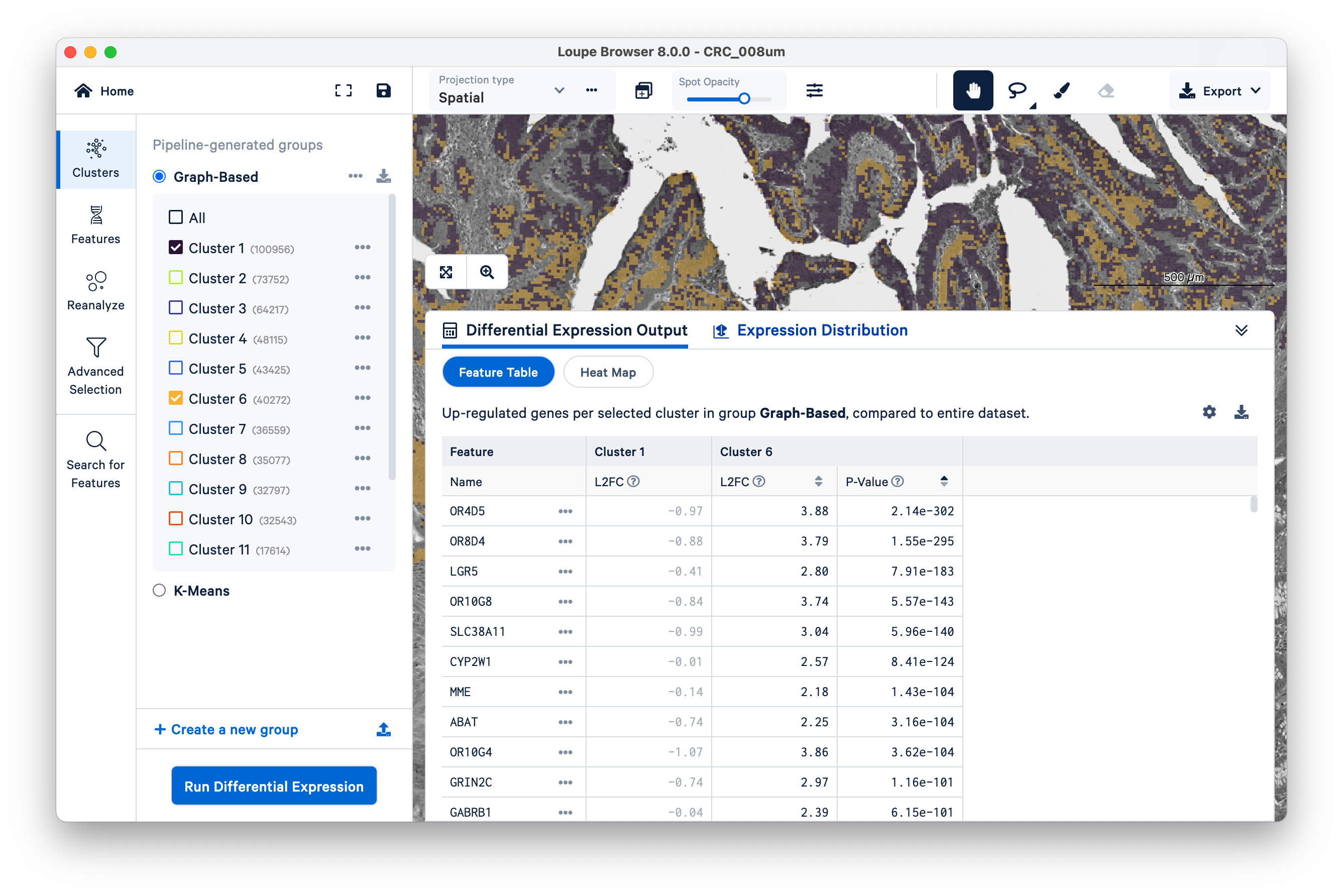
Expand the Differential Expression Output panel on the bottom to see genes upregulated in these two clusters relative to the entire dataset. These values were pre-computed by Space Ranger and are already loaded into the Loupe file. You can click to rank genes by log2fold change (L2FC) or p-value in each cluster.
Optionally, take some time to explore the other marker genes provided for macrophages and neutrophils.
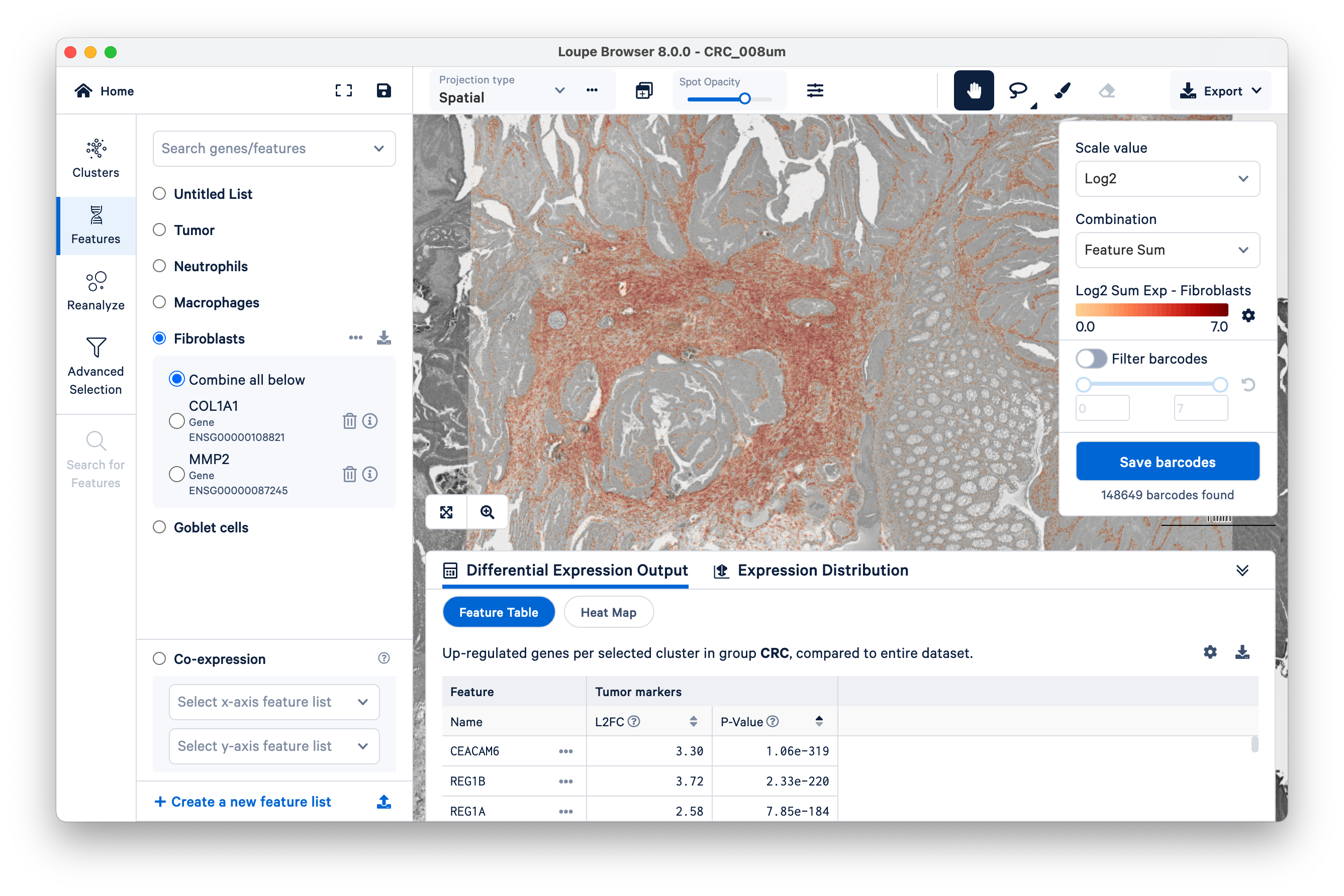
Next, we illustrate how to use our tumor marker genes to define a new group and then perform differential gene expression (DGE). Start by switching to Features, then filter “barcodes” (read “bins”) under a linear scale with a minimum of two UMIs.
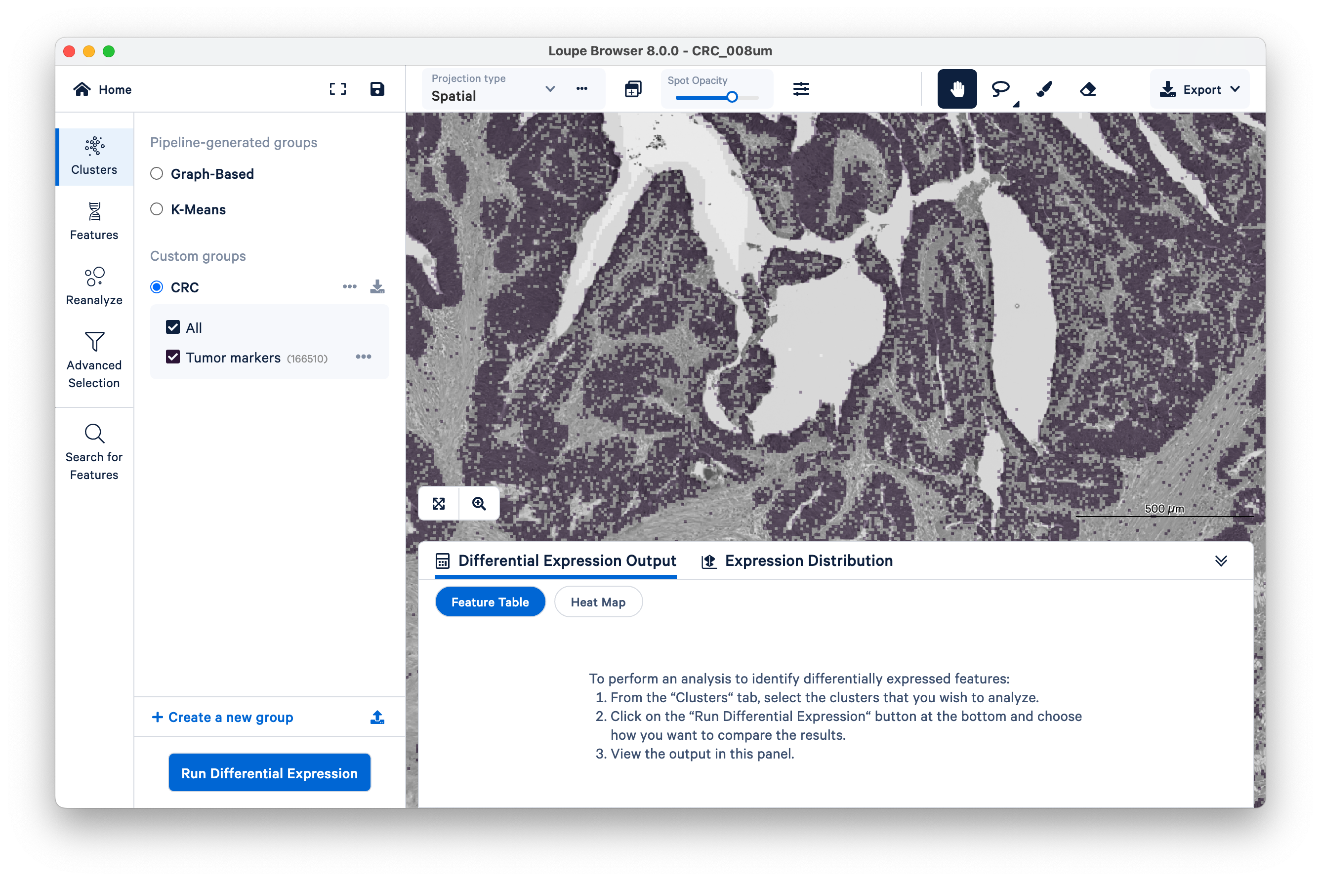
Name a new cluster (“Tumor Markers”), add to a new group (“CRC”), and click Finish.
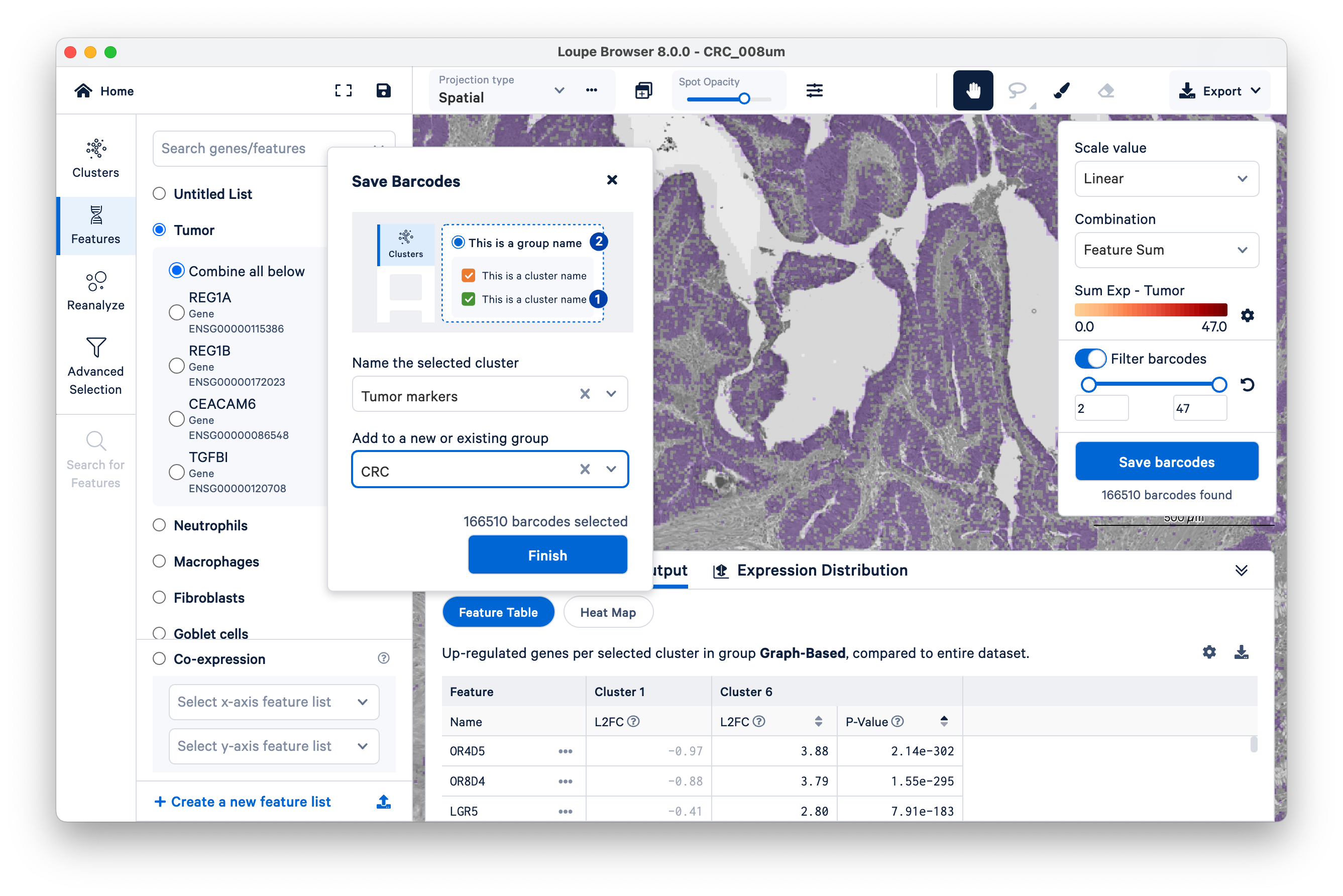
You will see your new group appear on the left-hand side under Clusters. Next, click Run Differential Gene Expression.
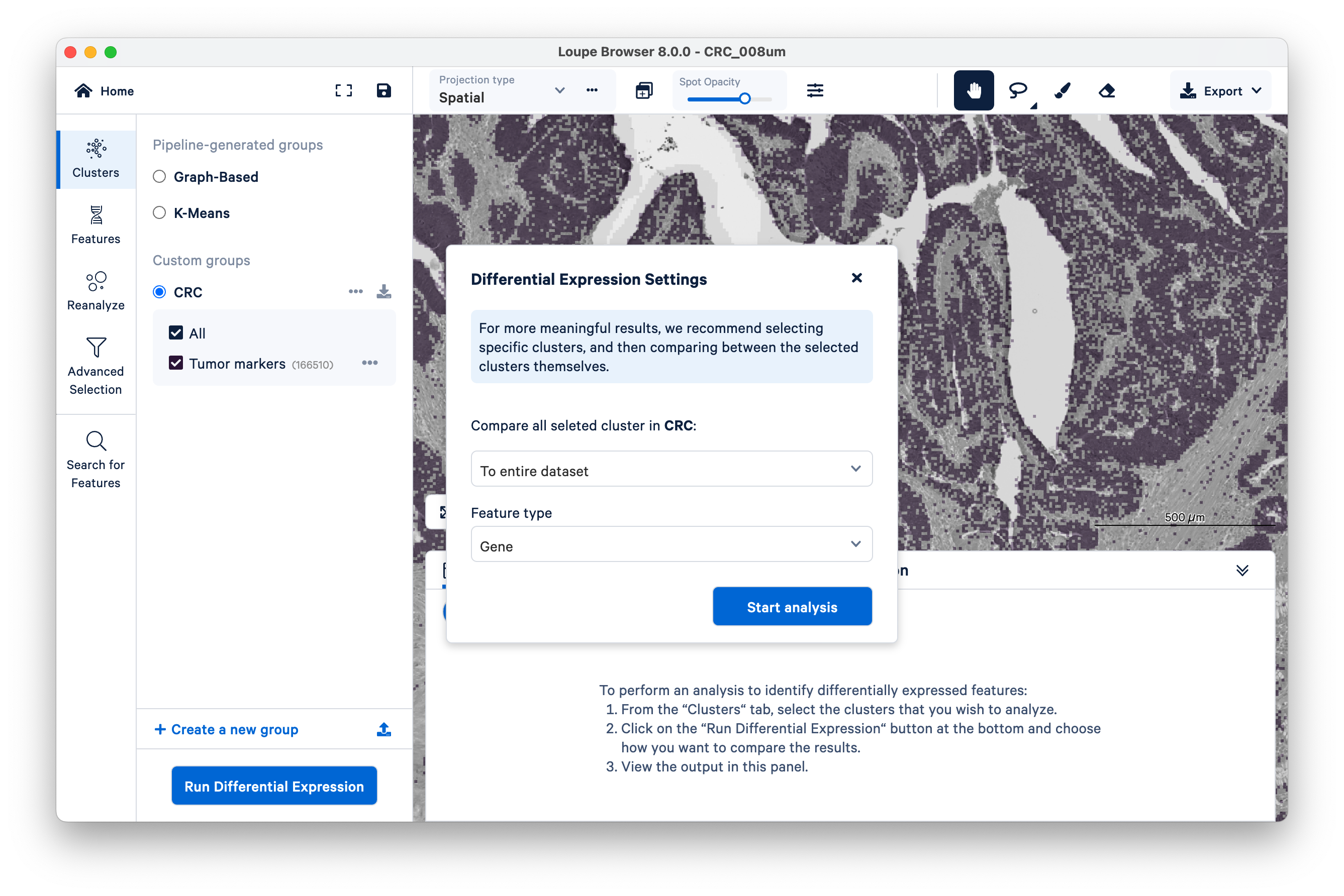
In this example, we compare our tumor cluster to the entire dataset, by gene.
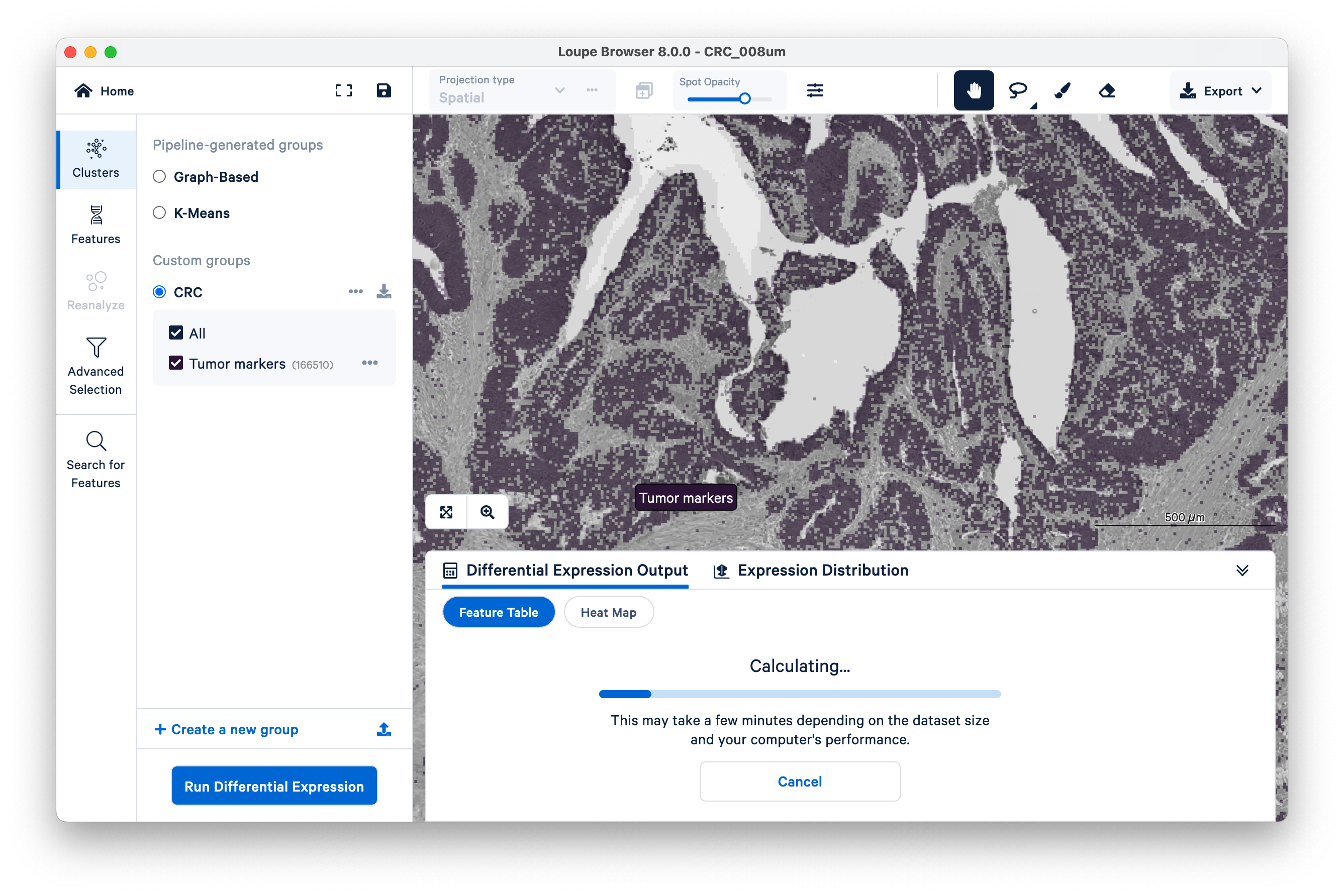
Loupe will show its progress as it runs the DGE.
When the analysis finishes, you can see the output. Unsurprisingly, we see genes like REG1A and REG1B (which were used to define the cluster in the first place), but as this is a whole-transcriptome assay, there are many other genes also upregulated alongside them.
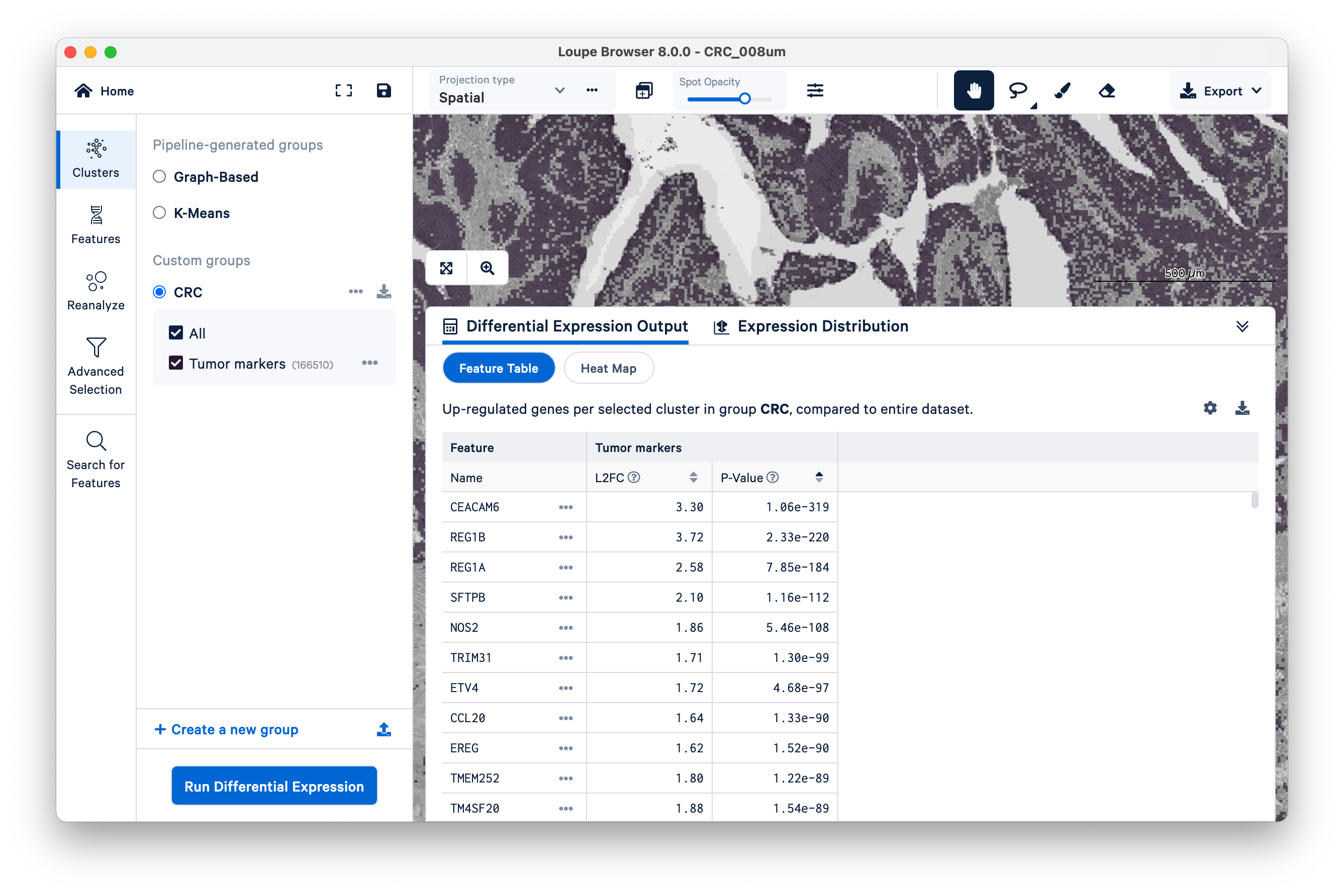
In this way, Visium HD data can be used as a discovery tool for new markers.
We conclude this tutorial by showcasing a the co-expression feature introduced in Loupe v8.0.
Start by viewing the co-expression of fibroblast and tumor markers. Notice the location of fibroblast markers using the Features view.
Next, on the bottom left, select the fibroblasts and tumor. You can now visualize both sets of gene markers together and use similar filters as described above, albeit for two gene lists at once.
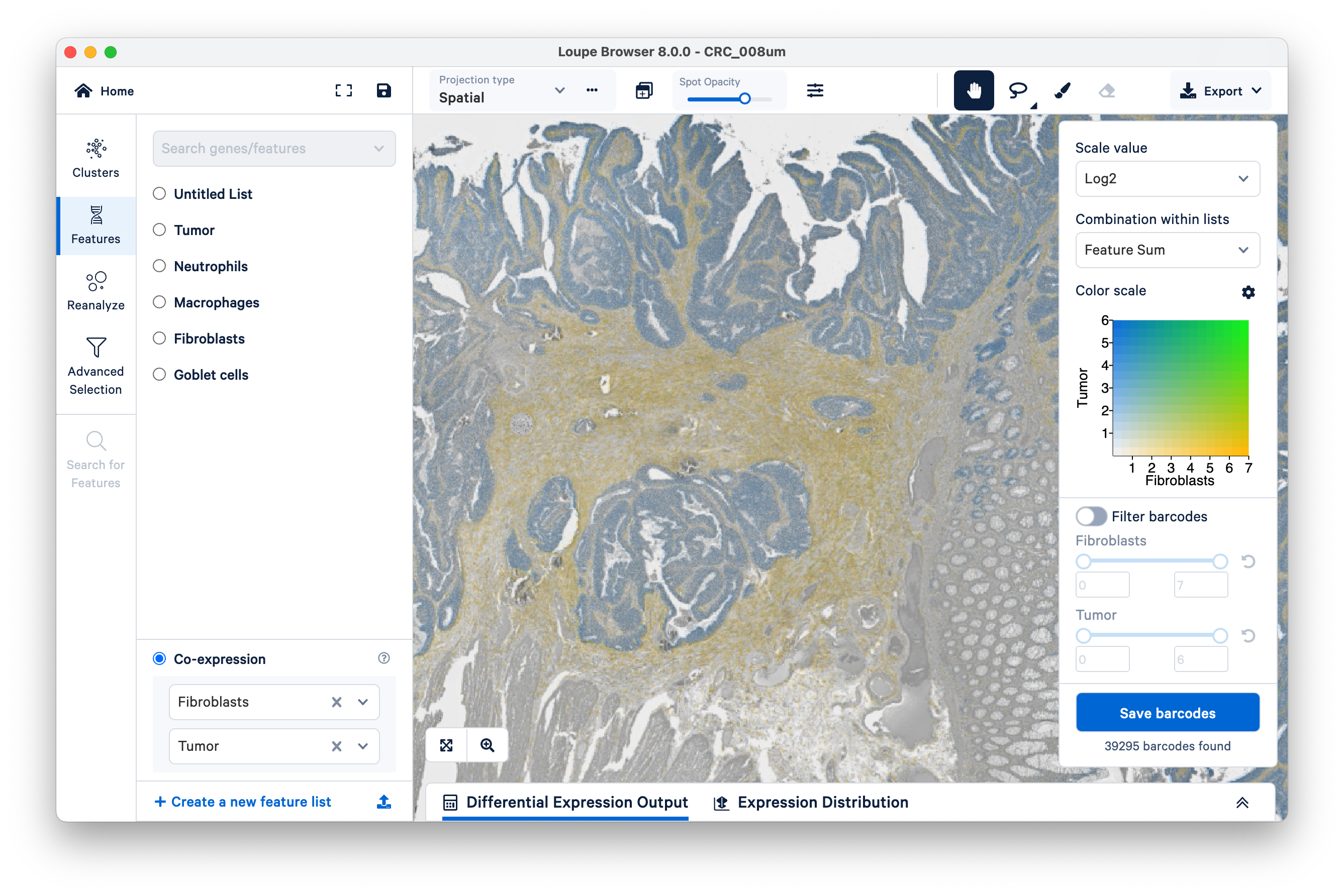
Note that tumor markers and fibroblasts are not co-expressed anywhere in the tissue (there is no visible green).
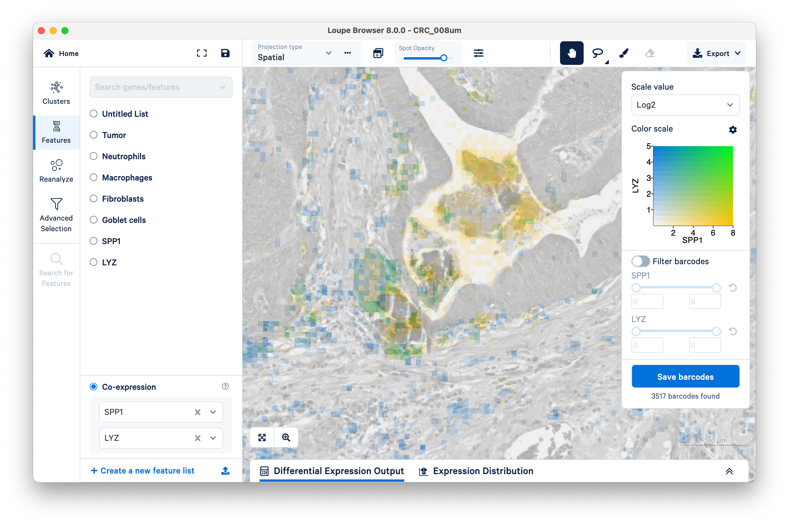
Contrast this pattern with LYZ (a general macrophage marker) and SPP1 (specific to SPP1+ macrophages). You will need to create a separate feature list for each gene.
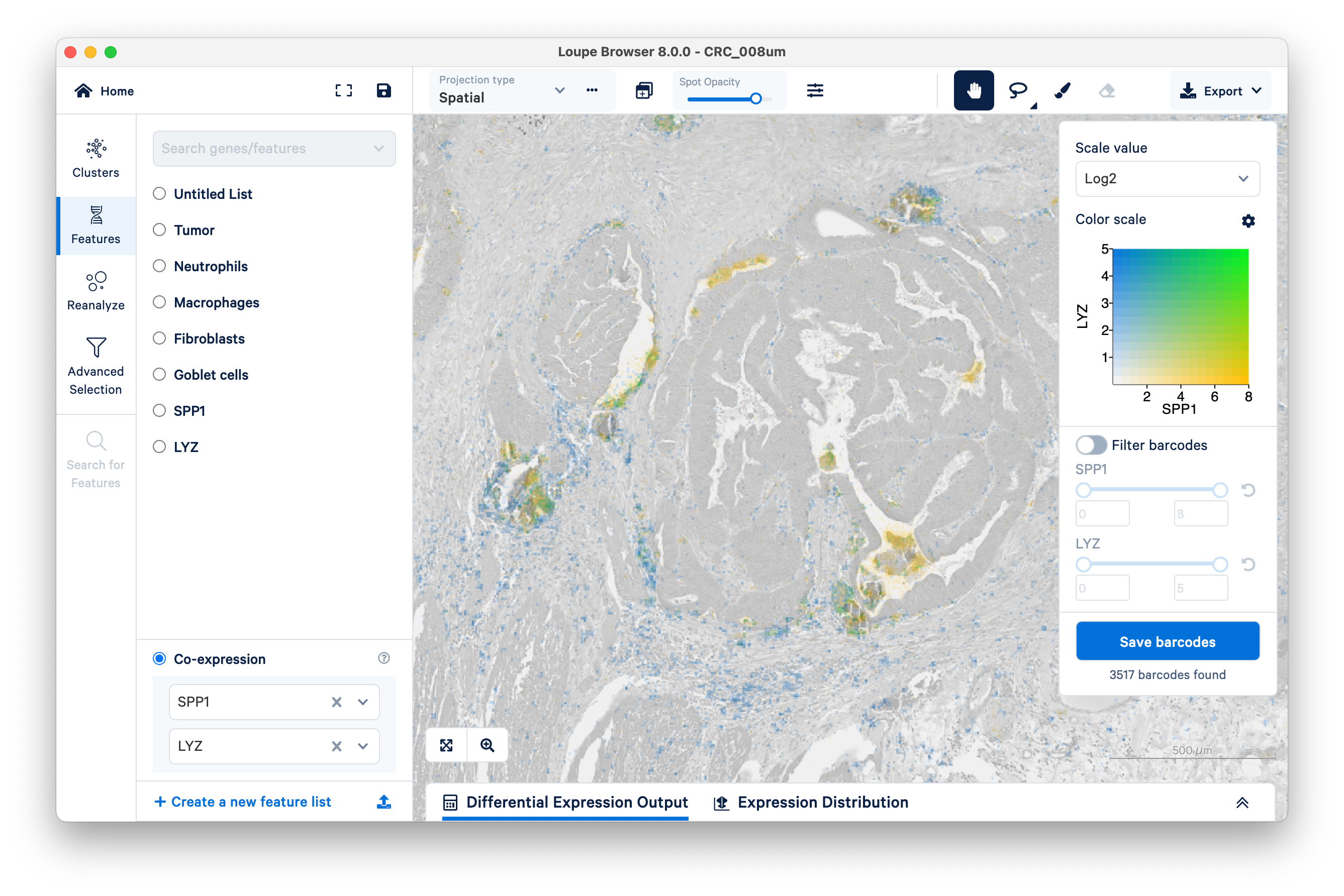
Unlike the previous example comparing the expression of fibroblasts vs. tumor, with SPP1 and LYZ macrophages, we can see areas of co-expression shown in green.
Analyzing large datasets like this one can be challenging with third party tools, which often require considerable skills in R, python, or other programming languages. In this tutorial we demonstrated how Loupe Browser makes it easy to get started exploring the biology of your sample without needing to write any code. You can zoom in and out seamlessly from the whole-tissue view to view 8 µm bins. You can quickly toggle between visualizing unsupervised clustering results and specific marker genes, or combinations of marker genes. You can run differential gene expression on the fly, and use these features in combination to map the whole transcriptome of the tumor microenvironment at high resolution.