How single cell sequencing data analysis works

Editor’s note: The purpose of this piece is to introduce how scRNA-seq data analysis works. Some steps have been simplified for clarity. If you are looking to understand the wet-lab workflow of an scRNA-seq experiment, we recommend you check out the first part of this series, “How does single cell RNA-sequencing work.” For comprehensive technical details, we recommend consulting the Software Support section of the 10x Support Hub.
The journey from sequencing library to data insights
The generation of a sequencing-ready library marks the end of messenger RNA’s (mRNA) physical “life” in a single cell RNA sequencing (scRNA-seq) experiment, but the journey is far from over. Once sequenced, RNA enters its “digital” life on the computational stage.
The transformation of scRNA-seq libraries into data outputs, like cell annotations and cluster graphs, is equally fascinating. For many new users, these parts of the single cell sequencing data analysis process can seem intimidating.
Not to worry! This article breaks down the inner workings of these steps to highlight how they help bring your single cell data to life. The key topics discussed are:
- Next-generation sequencing
-
Raw scRNA-seq data processing
- FASTQ file generation and explanation
-
Primary analysis
- Cell-feature matrix generation
- Quality filtering
-
Secondary and tertiary analysis
- Dimensionality reduction
- Clustering
- Cell annotation
- Differential gene expression
Chronicling the “digital” life of an mRNA molecule during scRNA-seq data analysis
Next-generation sequencing
For optimal sequencing, it is essential to perform a quality control (QC) assessment to accurately determine the library size distribution and concentration for loading the sequencer. The 10x Genomics Sequencing Handbook breaks down the QC process and recommends loading concentrations and sequencing parameters for a variety of sequencers. The libraries can then be diluted and loaded onto your sequencer.
We are now ready to turn our physical library molecules into digital sequencing readouts. Illumina’s next-generation sequencing (NGS), which we will focus on in this article for simplicity, uses the sequencing by synthesis (SBS) method to construct reads. In short, the library strands attach to oligos on the flow cell, and a complementary strand is synthesized. The length of your read depends on how many cycles are performed, and is limited by the length of the insert. Consult the user guide for your assay of choice or the 10x Genomics Sequencing Handbook for cycle recommendations.
Importantly, during Illumina sequencing, fluorescently labeled nucleotides are used to obtain the sequence of the library molecule over a series of imaging cycles (1). The photons emitted by the fluorescent labels, following excitation by the light source, are captured by a detector and recorded in Base Calling Files (BCL files)—marking the transition from a physical to a digital entity. Pretty neat, huh?
Before proceeding to the initial computational steps, it’s important to discuss the key components of your sequencing files. Illumina runs produce four reads: i5, i7, R1, and R2. To make sense of these designations, let’s revisit the single cell gene expression libraries that served as the sequencing input (Figure 1).
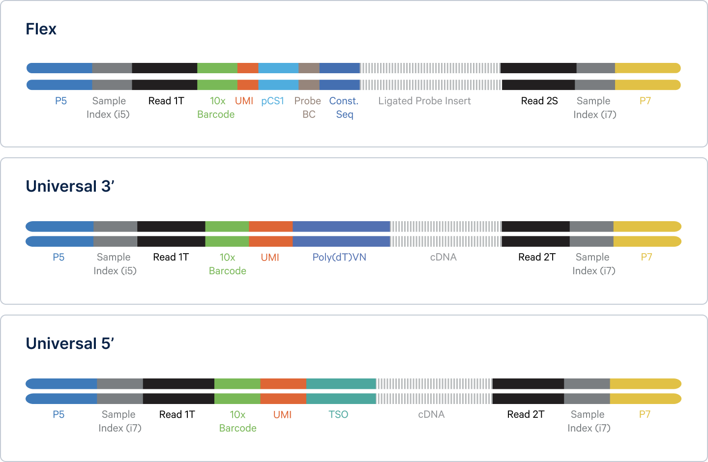
- The P5 and P7 sequences serve as attachment sites to the flow cell surface during the NGS run. They also contain primer binding sites that allow for the Sample Index reads (i5) and (i7) to be obtained. These reads enable multiple samples to be mixed in a single sequencing run, a process known as multiplexing, so that they can be distinguished from one another during data analysis (2). For simplicity, this post will not delve into the process of computational demultiplexing.
- The Read 1T sequence acts as a binding site for a primer that allows for determination of the R1 sequence. The Read 2T (Universal assays) and 2S (Flex assay) sequences act as binding sites for a primer that provides the sequences of R2 nucleotides and also of the insert, which gives us the identity of the original mRNA transcript. Spoiler: we’ll have more on these later.
Raw scRNA-seq data processing
FASTQ breakdown and file generation
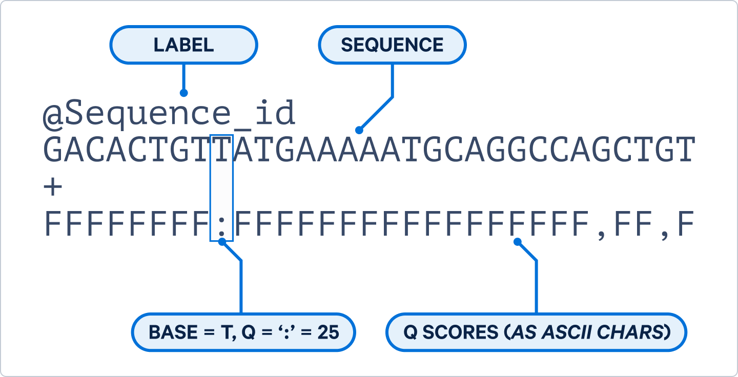
To start working with the sequencing data, the BCL file must first be converted to the FASTQ format. FASTQ is the standard format for storing raw scRNA-seq sequencing data, which includes the nucleotide sequences along with their associated quality scores (3). In this article, we will focus on the R1 and R2 FASTQ files only.
Within the sequences contained in the R1 files, the first ~16 bases correspond to the 10x Barcode (used to trace RNAs back to their cell of origin) and the following ~10–12 bases represent the unique molecular identifier (UMI; used for “counting” of transcripts to make sure the same RNA molecule is not counted multiple times). The subsequent bases correspond to the ligated probe insert (Flex assays) or complementary DNA (Universal assays).
The sequences in the R2 files will contain the sequence of the ligated probe insert (for Flex assays) or complementary DNA (for Universal assays). These sequences reflect the gene expression information for the original mRNA transcript, now in its digital form. For the next steps to proceed smoothly, it is critical to order these files so that all the IDs in the R1 file match the same line as the corresponding IDs in the R2 file.
Primary analysis
Cell-feature matrix generation

The ordered R1 and R2 files can now be used as inputs for the 10x Genomics Cell Ranger analysis pipeline. The fundamental output of this analysis is a cell-by-gene matrix, referred to as a cell-feature matrix in 10x analysis pipelines since the assay may be reporting something other than gene counts (e.g., antibody or CRISPR guide capture). In essence, Cell Ranger analysis maps reads to a reference to determine the identity of the transcripts and determines which cells they belong to based on the shared barcodes.
Before the cell-feature matrix generation can occur, we need to know what genes are expressed in your sample, a process known as alignment. The sequences in your R1 and R2 files are mapped onto a reference transcriptome matching your sample’s species. (Note: you’ll need a reference bundle generated from a reference genome FASTA file and a GTF file containing the transcript annotations. Similarly, our Flex assay needs the probe reference.)
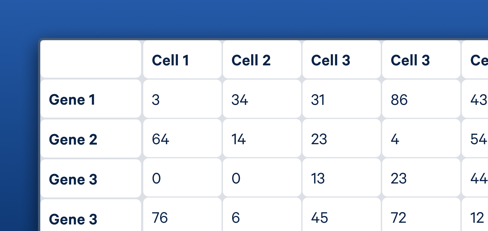
Now that we have identified what genes are present, we want to know how many molecules we sequenced for each gene. This is achieved by counting the number of unique barcode–UMI combinations, as each entity in the library is tagged with a UMI specific to its molecule and a 10x Barcode specific to its cell of origin. This information is presented as a matrix, with genes represented in the rows and barcodes in the columns.
It is worth noting that you get two matrices. One is a raw matrix that contains all the data. The second is a filtered matrix, which has removed the columns deemed not to represent true cells based on their RNA profiles. You can dive into the details of how this process is performed on the Cell Ranger’s Gene Expression Algorithm page. The filtered matrix file is what will be used for subsequent analysis.
Quality filtering
After processing your raw data with the Cell Ranger pipeline, you should review the summary file as a first-pass QC check for each sample. This check will help you identify whether you want to filter further before downstream analysis or if there were potential issues with the sample prep or experiment setup.

Single cell data analysis has never been so fast and simple
We understand how overwhelming scRNA-seq data analysis can seem, especially without bioinformatics experience. With 10x Genomics Cloud Analysis, you gain the power of our Cell Ranger pipeline through a fast and intuitive web interface, no need for command-line experience.
Secondary and tertiary analysis
Dimensionality reduction
Given the size of transcriptomes, it should come as no surprise that the filtered cell-feature matrix contains a lot of data. Lots of data means a heavy computational burden, which is why it is standard for single cell analysis to include dimensionality reduction.
Essentially, this process finds the most important patterns and condenses the data down into something more manageable. Furthermore, it simplifies data visualization and provides more robust, less noisy representations. Several common dimensionality reduction techniques are described briefly below:
- Principal Component Analysis (PCA): PCA identifies the principal components (PCs) that account for the most variance in your data. It is widely used in scRNA-seq bioinformatics as an initial denoising and data compression step that generates the inputs for t-SNE or UMAP generation (described below).
- t-Distributed Stochastic Neighbor Embedding (t-SNE) and Uniform Manifold Approximation and Projection (UMAP): A simple way to think of these methods is that they group similar cells together in a 2D or 3D plot to help you visual high-dimensional datasets, such as those you get from single cell experiments.
Note: While UMAPs are more commonly published, there's some debate in the field about how to best describe the differences in what you learn from a UMAP versus a t-SNE (4). It's often helpful to generate and review both visualizations during your analysis.
More information on how the Cell Ranger pipeline achieves this can be found on the Cell Ranger support page.

Become a bioinformatics pro with our Analysis Guides
Grow your bioinformatics skills from foundational concepts to advanced techniques. Our Analysis Guides feature a collection of introductions, step-by-step tutorials, and blogs that provide data analysis guidance using 10x Genomics and community-developed software tools, enabling you to achieve deeper explorations of your data.
Clustering
While your eyes may perceive groupings in t-SNEs and UMAPs, the groupings you see are based on a 2D rendering. However, there is really no concept of where one group begins and another ends in these visualizations. For that, you need to perform clustering, which goes back to the PCA-reduced data and computationally groups cells based on similar gene expression profiles.
You know those colorful t-SNEs and UMAPs that you see in publications? This is where the colors come from. These clusters may represent distinct cell types, but they could also be influenced by subtypes or cellular states.
Common clustering algorithms include:
- K-means: This method partitions data into a user-specified number (k) of clusters. It is often useful as an initial data assessment. For example, it can help you quickly determine if predefined experimental conditions, such as the control and treatment groups, segregate into distinct clusters by specifying k = 2.
- Graph-based clustering: This method partitions data into clusters based on the data's structure rather than a predefined number. The number of clusters you get from this approach will vary a bit depending on the parameters set. It’s a good way to quickly identify potential cell types or states you may not have been expecting.
Specific details of how the Cell Ranger pipeline performs these methods can be found on the Cell Ranger support page.

Intuitively visualize and explore your scRNA-seq data
Loupe Browser is a powerful visualization software that provides the intuitive functionality you need to explore and analyze your Chromium single cell data. Uncover and plot differentially expressed genes, rapidly identify the expression of your genes of interest, quickly create high-resolution figures, and more.
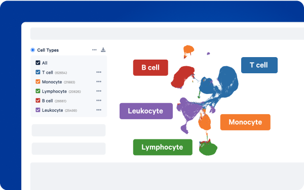
Cell annotation
If you are looking to understand what cell types are present within your sample—and how those relate to your clusters—then you will need to annotate your cells. This step can be done manually by looking for known marker genes in each cluster, or it can be automated using computational algorithms that leverage curated gene sets or reference datasets to assign meaning to the RNA expression profile of each cell in your data.

Reduce the burden of manual annotation
Get a jumpstart on your single cell insights. Our Automated Cell Annotation feature—available in 10x Cloud Analysis and Cell Ranger versions 9.0.0 and higher—automatically identifies and annotates both broad and fine-grain human cell types based on standardized single cell datasets.
Differential gene expression
Once you get to this point, there are a number of different kinds of analysis you can do. Differential expression (DE) analysis is one of the more common options and can be helpful in answering a variety of questions.
If you are manually annotating your cells, DE can help you identify potential marker genes that identify your clusters as specific cell types. If you are comparing different disease states or treatment conditions, DE can help you understand how the RNA expression profiles changed between experimental groups (i.e., which genes are significantly up- or downregulated in each cluster compared to others). DE analysis is performed by default in the Cell Ranger pipeline and can be customized for your experiment in the Loupe Browser software.
RNA’s journey from experimental design to data discovery
From raw FASTQ files to annotated cell clusters or differential gene expression results, each computational step helps unlock the biological meaning the RNA molecule contained. While single cell sequencing data analysis may seem daunting at first, understanding the logic behind each stage makes them easier to approach with confidence.
Before wrapping up, we would be remiss not to mention that your data analysis journey begins before you even pick up a pipette and can continue beyond the analyses covered here. The choices you make when designing your experiment can either enable or rule out the kinds of analysis you can do. For example, to perform statistically sound differential expression analysis, it is important to have an appropriate sample size. Further down the workflow, sample collection and processing can diminish or create batch effects.

Likewise, the data analysis journey doesn’t necessarily end here. As new analysis methods are developed or additional questions come up, our trusty RNA molecule is ready to help move science forward in its immortalized digital state.

Curious about bringing single cell to your lab?
Single cell sequencing is uniquely poised to unlock the cellular underpinnings driving the biology you are looking to understand. 10x Genomics is making scRNA-seq more accessible than ever with an end-to-end platform that simplifies every step—from sample prep to data analysis. If you’re ready to bring these powerful advantages to your lab, we’re here to help you figure out the right solutions for you.
References:
- Bentley D, et al. Accurate whole human genome sequencing using reversible terminator chemistry. Nature 456: 53–59 (2008). doi: 10.1038/nature07517
- “Overview of Illumina Chemistry.” Resources, MGH NextGen Sequencing Core, nextgen.mgh.harvard.edu/IlluminaChemistry.html. Accessed 9 July 2025.
- “Quality Scores.” BaseSpace Sequence Hub, Illumina, Inc., help.basespace.illumina.com/files-used-by-basespace/quality-scores. Accessed 9 July 2025.
- Marx V. Seeing data as t-SNE and UMAP do. Nat Methods 21: 930–933 (2024). doi: 10.1038/s41592-024-02301-x
About the author: