cellranger aggr does not support Targeted Gene Expression and LT libraries.Many experiments generate data for multiple samples. Depending on the experimental design, these samples may represent replicates from the same set of cells, cells from different tissues or time points from the same individual, or cells from different individuals. These samples could be processed through various Gel Bead-in Emulsion (GEM) wells wells or multiplexed within the same GEM well on Chromium instruments.
The cellranger count, cellranger vdj, and cellranger multi pipelines are designed to process data from a single GEM well. To work with data from multiple GEM wells, you can aggregate and analyze the outputs from multiple runs of each of these pipelines using cellranger aggr.
cellranger aggr is NOT designed for aggregating multiple sequencing runs of the same library, for example, resequencing the same library to increase read depth. In this scenario, you must specify all FASTQ files (fastqs field) in a single analysis of either cellranger count or multi.The first step is to run cellranger count, cellranger vdj, or cellranger multi on each individual GEM well prepared using a 10x Genomics Chromium instrument.
For example, if you ran the cellranger count pipeline three times:
cd /opt/runs
cellranger count --id=LV123 ...
... wait for pipeline to finish ...
cellranger count --id=LB456 ...
... wait for pipeline to finish ...
cellranger count --id=LP789 ...
... wait for pipeline to finish ...
These three runs can be aggregated using cellranger aggr to obtain a unified feature-barcode matrix and secondary analysis outputs.
The cellranger aggr pipeline gets information on which libraries you wish to aggregate from an input file called the aggregation CSV.
Change in aggregation CSV column headers:
Starting with Cell Ranger v6.0 and Loupe Browser v5.1.0: sample_id,molecule_h5
Prior versions: library_id,molecule_h5
The aggregation CSV looks slightly different depending on whether or not your experiment includes a V(D)J library (5' Immune Profiling workflow). The different sections below will help you find the aggregation CSV suitable for your experimental design.
You can either make the aggregation CSV file using a text editor or create it in Excel and save as a CSV file.
Gene Expression (with or without Feature Barcode) libraries from a single GEM well can be analyzed using either cellranger count or cellranger multi. The cellranger aggr command takes an aggregation CSV file specifying the list of either cellranger count or multi output files (specifically the molecule_info.h5 from each run), and produces a single feature-barcode matrix containing all the data.
When combining multiple GEM wells, the barcode sequences for each channel are distinguished by a GEM well suffix appended to the barcode sequence (see GEM wells).
By default, reads from each GEM well are subsampled such that all GEM wells have the same effective sequencing depth, measured in terms of reads that are confidently mapped to the transcriptome or assigned to the feature IDs per cell. However, it is possible to change the depth normalization mode (see Depth Normalization).
The CSV header line should contain the following columns:
| Column name | Description |
|---|---|
sample_id | Unique identifier for this input GEM well. This will be used for labeling purposes only; it does not need to match any previous ID assigned to the GEM well. |
molecule_h5 | Path to the molecule_info.h5 or sample_molecule_info.h5 file produced by cellranger count or multi, respectively. For example: If you processed your GEM well by calling cellranger count --id=ID in a directory called /DIR, this path would be /DIR/ID/outs/molecule_info.h5. If you processed your GEM well by calling cellranger multi for Cell Multiplexing data by calling cellranger multi --id=ID in a directory called /DIR, and the sample was called Sample1, this path would be /DIR/ID/outs/per_sample_outs/Sample1/sample_molecule_info.h5 |
count
An example aggregation CSV for samples processed using cellranger count
sample_id,molecule_h5
LV123,/opt/runs/LV123/outs/molecule_info.h5
LB456,/opt/runs/LB456/outs/molecule_info.h5
LP789,/opt/runs/LP789/outs/molecule_info.h5
multi
Here is an example aggregation CSV for samples processed using cellranger multi:
sample_id,molecule_h5
Sample1,/opt/runs/Run1/outs/per_sample_outs/Sample1/sample_molecule_info.h5
Sample2,/opt/runs/Run1/outs/per_sample_outs/Sample2/sample_molecule_info.h5
If your experiment includes V(D)J libraries generated using the 5' Immune Profiling workflow, cellranger aggr uses the vdj_contig_info.pb from each cellranger vdj and/or cellranger multi run to aggregate the data and perform clonotype grouping.
Both cellranger vdj and cellranger multi (for experiments that include a V(D)J library) runs will generate these vdj_contig_info.pb output files. However, the location of the file differs based on the pipeline:
cellranger vdjoutputs thevdj_contig_info.pbin a folder similar to:/DIR/ID/outs/vdj_contig_info.pbcellranger multioutputs thevdj_contig_info.pbin theper_sample_outsfolder with a path similar to:/DIR/ID/outs/per_sample_outs/Sample1.
Since the paths are different for vdj vs. multi outputs, the aggregation CSVs also look different. If you wish to aggregate outputs that were run with a combination of cellranger vdj and cellranger multi, see the Special cases section below.
vdj
The aggregation CSV used to aggregate cellranger vdj outputs needs the following columns:
| Column Name | Description |
|---|---|
sample_id | Unique identifier for this input GEM well. This will be used for labeling purposes only; it does not need to match any previous ID assigned to the GEM well. |
vdj_contig_info | Path to the contig info file produced by cellranger vdj. For example, if you processed your GEM well by calling cellranger vdj --id=ID in a directory named /DIR, this path would be /DIR/ID/outs/vdj_contig_info.pb |
donor | A donor is an individual from whom adaptive immune cells (T cells, B cells) are collected (e.g. a sister and a brother would each be considered unique donors for the purposes of V(D)J aggregation). |
origin | The origin is the specific source from which a dataset of cells is derived. This could be a timepoint (pre- or post-treatment or vaccination or time A/B/C), a tissue (PBMC, tumor, lung), or other metadata (healthy, diseased, condition). Origins must be unique to each donor. Replicates (e.g. multiple libraries from the same population of cells) may share origins within a donor, which triggers additional replicate-based filtering. |
How are donor and origin values used in aggr?
- If two datasets come from the same donor but have different origins, Cell Ranger will rerun the clonotype grouping algorithm on the combined set of cells. This allows cells from different datasets to belong to the same clonotype.
- If two datasets come from the same donor and origin, then Cell Ranger performs additional filtering to remove certain rare artifacts. For example, Cell Ranger will filter expanded exact subclonotypes that are present in one library but not in another from the same origin, which would be highly improbable, assuming random draws of cells from the tube. These are believed to arise when a plasma or plasmablast cell breaks up during or after pipetting from the tube, and the resulting fragments contaminate GEMs, yielding expanded false clonotypes that are residues of real single plasma cells.
- If two cells came from different donors, then Cell Ranger will not put them in the same clonotype.
In addition to the CSV columns expected by cellranger aggr, you may optionally supply columns containing library metadata (e.g., lab or sample origin). These custom library annotations do not affect the analysis pipeline but can be visualized downstream in Loupe Browser (see Categories section below).
Required columns and experimental design information are shown here:
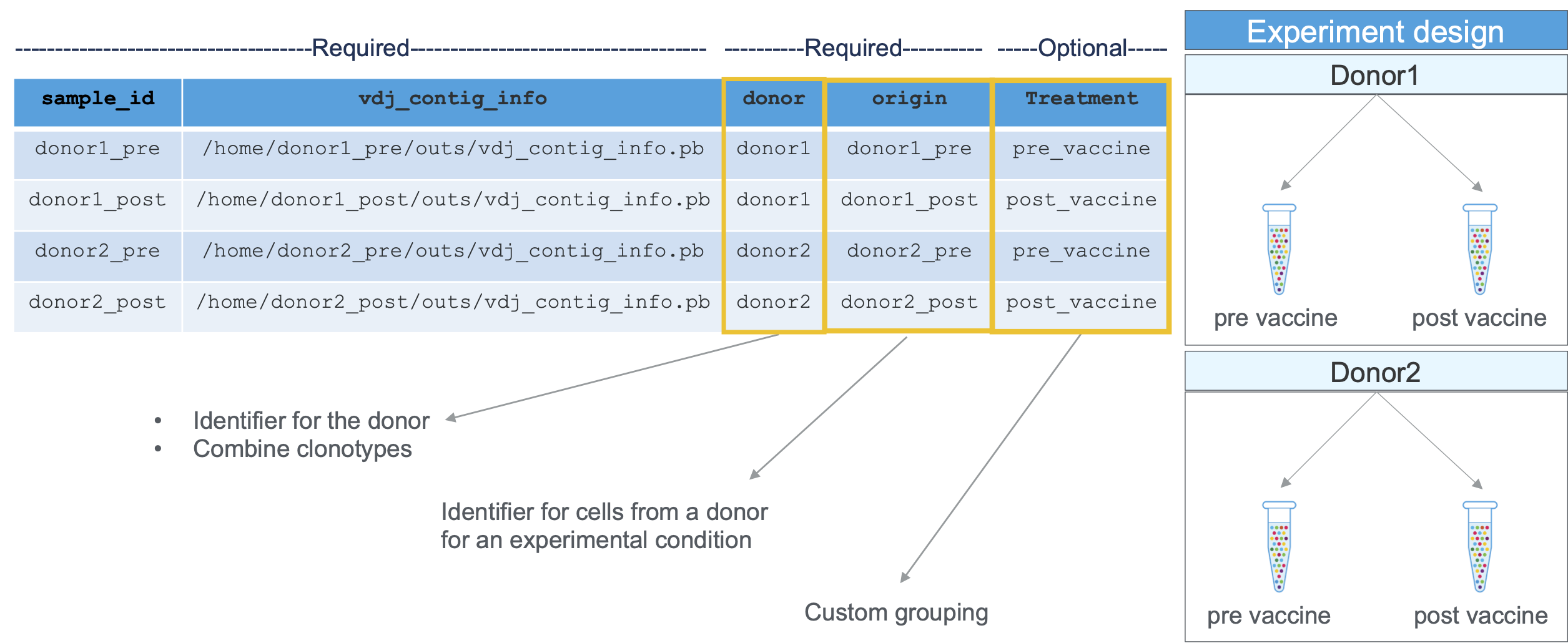
An example aggregation CSV for samples processed using cellranger vdj (including a custom column called 'VaccinationStatus'):
sample_id,vdj_contig_info,donor,origin,VaccinationStatus
Sample1,/opt/runs/Lib1/outs/vdj_contig_info.pb,D1,pbmc_t0,Pre-Vaccination
Sample2,/opt/runs/Lib2/outs/vdj_contig_info.pb,D1,pbmc_t1,Post-Vaccination
The pipeline will produce an error if the individual libraries were run using different V(D)J references or if the chain type (TCR or IG) in the individual libraries is inconsistent.
multi
The cellranger aggr command can take a CSV file specifying a list of cellranger multi output directories, and perform aggregation on any combination of 5' Gene Expression, Antibody Capture, CRISPR, and V(D)J libraries that are present in the individual runs of cellranger multi.
However, ALL the runs of cellranger multi included in the aggregation CSV must have the same combination of libraries. For example, if Sample1 has Gene Expression, BCR, and TCR, whereas Sample2 has only Gene Expression and BCR, cellranger aggr fails with this error message:
[error] Pipestance failed. Error log at:
path/to/error_message/chnk0-u4933b35480/_errors
Log message:
The multi outs folders supplied as inputs to aggr contain an inconsistent set of libraries:
- 'Sample1' contains [count, vdj_t, vdj_b]
- 'Sample2' contains [count, vdj_b]
To aggregate `multi` outputs, all the individual inputs must contain the same set of library types. If you would like to use `aggr` for only one library type, you can supply the respective `molecule_info` (for `count`) or the `vdj_contig_info` (for `vdj`)
The aggregation CSV used to aggregate cellranger multi outputs needs the following columns:
| Column Name | Description |
|---|---|
sample_id | Unique identifier for this input GEM well. This will be used for labeling purposes only; it does not need to match any previous ID assigned to the GEM well. |
sample_outs | Path to the per_sample_outs folder generated by cellranger multi. For example, if you processed your GEM well by calling cellranger multi --id=ID --csv=exp1.csv in a directory called /DIR , and the sample was called Sample1, this path would be /DIR/ID/outs/per_sample_outs/Sample1 |
donor | A donor is an individual from whom adaptive immune cells (T cells, B cells) are collected (e.g. a sister and a brother would each be considered unique donors for the purposes of V(D)J aggregation). |
origin | The origin is the specific source from which a dataset of cells is derived. This could be a timepoint (pre- or post-treatment or vaccination or time A/B/C), a tissue (PBMC, tumor, lung), or other metadata (healthy, diseased, condition). Origins must be unique to each donor. Replicates (e.g. multiple libraries from the same population of cells) may share origins within a donor, which triggers additional replicate-based filtering. |
Note that the column header vdj_contig_info is replaced by sample_outs for cellranger multi runs.
The cellranger aggr pipeline will auto-detect the presence of various libraries based on the structure and contents of the per sample outs folders. Besides the change in the input CSV column (sample_outs instead of molecule_h5 or vdj_contig_info), other aspects (depth normalization, batch correction, etc.) of the algorithm remain the same.
An example aggregation CSV for two 5' Immune Profiling samples processed using cellranger multi:
sample_id,sample_outs,donor,origin
Sample1,/opt/runs/Sample1/outs/per_sample_outs/Sample1,D1,pbmc_t0
Sample2,/opt/runs/Sample2/outs/per_sample_outs/Sample2,D1,pbmc_t1
If Feature Barcode analysis is included, the input Feature Reference CSV file should be the same for each GEM well.
CRISPR Guide Capture
Starting with Cell Ranger v7.0, CRISPR Guide Capture libraries from multiple GEM wells can be aggregated using cellranger aggr. There are no changes to aggr inputs – the presence of CRISPR Guide Capture library information in the molecule_info.h5 input files enables CRISPR aggregation. Normalization is enabled by default for both Gene Expression and CRISPR Guide Capture libraries; changes to normalization parameters affect both libraries.
Protospacer calling is performed again on the combined data included in the cellranger aggr run. The process of aggregating CRISPR data generates a crispr_analysis/ folder within the outs/ directory. The structure of the crispr_analysis folder folder resembles the CRISPR outputs produced by cellranger count or cellranger multi.
Antigen Capture (BEAM)
Starting with Cell Ranger v7.2, cellranger aggr can be used to aggregate 5' Immune Profiling samples that include Antigen Capture libraries. cellranger aggr will combine and normalize the calculation of antigen specificity scores across multiple or large samples split across GEM wells.
When combining multiple samples into a single dataset with cellranger aggr, you can assign categories and values to individual samples by adding columns to the cellranger aggr input CSV. These category assignments carry over into Loupe Browser, where you can access them in Clusters Mode to help identify differentially expressed genes between samples.
Any columns in addition to sample_id and molecule_h5 will be converted into categories. Cells in each sample will be assigned to one of the values within that category.
Here is an example aggregation CSV where samples are categorized into 'treatment' and 'control' experiments. The new category is introduced as a column labeled 'experiment':
sample_id,molecule_h5,experiment
LV123,/opt/runs/LV123/outs/molecule_info.h5,control
LB456,/opt/runs/LB456/outs/molecule_info.h5,treatment
LP789,/opt/runs/LP789/outs/molecule_info.h5,treatment
Unlike other CSV inputs to Cell Ranger, these custom columns accept characters outside the ASCII range (e.g., non-Latin characters).
This section describes the most common command line arguments for aggr. Run cellranger aggr --help or visit the Cell Ranger command line arguments page for a full list.
| Argument | Description |
|---|---|
--id | Required. A unique run ID string: e.g. AGG123 |
--csv | Required. Path to the aggregation CSV file containing the list of molecule_info.h5 files. |
--normalize | Optional. String specifying how to normalize depth across the input libraries. Valid values: mapped (default) or none (see Depth Normalization). |
After specifying these input arguments, run cellranger aggr:
cd /home/jdoe/runs
cellranger aggr --id=AGG123 --csv=AGG123_aggr.csv
The pipeline will begin to run, creating a new output folder named with the specified aggregation ID (e.g. /home/jdoe/runs/AGG123). If this folder already exists, Cell Ranger will assume it is an existing pipestance and attempt to resume running it.
The cellranger aggr command can be used to aggregate outputs from a combination of cellranger multi and cellranger vdj runs. The aggregation CSV must have the column names described in the vdj section.
The path to the vdj_contig_info.pb file is required even for samples processed with cellranger multi. The vdj_contig_info.pb is located in the sample_outs/ directory with a path similar to /per_sample_outs/Sample1/vdj_b/vdj_contig_info.pb for a BCR library.
This example CSV is used to aggregate the outputs from a BCR library processed with cellranger multi and a BCR library processed with cellranger vdj:
sample_id,vdj_contig_info,donor,origin
Sample1,/opt/runs/Sample1/outs/per_sample_outs/Sample1/vdj_b/vdj_contig_info.pb,D1,pbmc_t0
Sample2,/opt/runs/Sample2/outs/vdj_contig_info.pb,D1,pbmc_t1
If you are aggregating libraries generated by different chemistry versions of the Single Cell Gene Expression Reagents, you might observe systematic differences in gene expression profiles between libraries. The cellranger aggr pipeline incorporates batch effect correction (algorithm details) to overcome this. To enable batch correction, include the following column in your aggregation CSV file:
- batch: Optional. Unique identifier for the batch that this GEM well belongs to. Libraries with the same batch identifier are considered to be in the same batch.
For example, if the LV123 sample in the previous example is a v2 library and the LB456 and LP789 samples are v3 libraries, set up the aggregation CSV file like this:
sample_id,molecule_h5,batch
LV123,/opt/runs/LV123/outs/molecule_info.h5,v2_lib
LB456,/opt/runs/LB456/outs/molecule_info.h5,v3_lib
LP789,/opt/runs/LP789/outs/molecule_info.h5,v3_lib
The v2_lib and v3_lib identifiers are example identifiers. Every sample from a given batch must have the same batch identifier, but otherwise, the identifier text itself is arbitrary.
About chemistry batch correction
- This Chemistry Batch Correction algorithm is specifically intended to correct for systematic variability in gene expression profiles caused by different versions of the Single Cell Gene Expression chemistry. 10x Genomics has tested and verified its effectiveness primarily on aggregating Single Cell Gene Expression v2 and v3 chemistry with well-matched input material. The algorithm may be useful in other scenarios but will require careful validation of results.
- Chemistry batch correction affects the PCA, t-SNE, and UMAP visualization and clustering results. Values in the aggregated feature-barcode matrix are not adjusted by chemistry batch correction. Differential expression analysis is still performed on the feature-barcode count matrix.
- When chemistry batch correction is enabled, FBPCA is used to perform dimensionality reduction instead of IRLBA PCA.
- The batch effect score (described in algorithm details) is recommended to compare the performance before and after batch correction. Besides the batch effect, the score also depends on the composition of the cell populations across batches.
- The minimum System Requirements of 64GB RAM will allow batch correction on datasets with a total number of 128k cells.
- Libraries with different throughput but the same chemistry can be aggregated without chemistry batch correction. For example, Single Cell 3' Gene Expression v3.1 standard kit (SK) and HT can be aggregated without batch correction, as can Single Cell 5’ Gene Expression SK and HT. See Knowledge Base article for details.
Aggregating Single Cell 5' and 3' Gene Expression data
The cellranger aggr pipeline uses Chemistry Batch Correction when aggregating results from a combination of 5' and 3', or 3' v2 and 3' v3 Gene Expression data. Enabling Chemistry Batch Correction in this scenario improves the mixing of the batches in the t-SNE visualization and clustering results. We recommend using Chemistry Batch correction for these scenarios, however, residual batch effects may still be present, and careful validation of the results is advised. In particular, for the V(D)J genes, the 5' Gene Expression assay will generally count the V gene segments of the immune receptor (e.g. TRBV12-1 or IGH4-2), while the 3' Gene Expression assay will count the C gene segments (e.g. TRBC or IGHA), which may pose additional analysis challenges.
The cellranger aggr pipeline supports the aggregation of Cell Multiplexing v3.1 data with Single Cell 3’ Gene Expression v3.1 data (i.e. "non-Cell Multiplexing data").
To combine Cell Multiplexing with non-Cell Multiplexing data, cellranger aggr (v6.0 and later) requires identical references (including feature/CMO reference). Therefore, non-Cell Multiplexing data must be re-run with the CMO reference file that specified Cell Multiplexing tags (CMOs) for the Cell Multiplexing data. These datasets can be run with either cellranger count (v3.0 and later) or cellranger multi (v5.0 and later). We recommend using the same version of Cell Ranger to generate inputs for cellranger aggr.
- Option 1) For
cellranger count, input the CMO reference with--feature-refand use the--no-librariesoption. Thecellranger countpipeline will generate amolecule_info.h5, which can be used as input to thecellranger aggrpipeline. An example of the command is below (customize the relevant file paths):
cellranger count --id=pbmc_1k_count \
--transcriptome=/path/to/transcriptome/GRCh38-2020-A \
--fastqs=/path/togex/fastqs/pbmc_1k_v3_fastqs/ \
--sample=pbmc_1k_v3 \
--feature-ref=/path/to/cmo-reference/cmo-ref.csv \
--no-libraries
- Option 2) For
cellranger multi, input the CMO feature reference in the[feature]section of the multi config CSV file. An example of the config file is below (customize the relevant file paths):
[gene-expression]
reference,/path/to/transcriptome/GRCh38-2020-A
create-bam,true
[feature]
reference,/path/to/cmo-reference/cmo-ref.csv
[libraries]
fastq_id,fastqs,feature_types
pbmc_1k_v3,/path/togex/fastqs/pbmc_1k_v3_fastqs/,Gene Expression
The cellranger multi pipeline generates a per sample sample_molecule_info.h5 file which is equivalent to the molecule_info.h5 file from a cellranger count run. These files can be used as input to the cellranger aggr pipeline. An example of the multi pipeline command is below (customize the relevant file paths):
cellranger multi --id=pbmc_1k_multi --csv=/path/to/config.csv
The Cell Multiplexing protocol has additional wash steps that may lead to the depletion of more ambient mRNA from samples compared to non-Cell Multiplexing samples. This difference in mRNA may then introduce small batch effects between Cell Multiplexing and non-Cell Multiplexing datasets. However, observations from internal data show fairly small batch effects, and batch effect correction is not needed in most cases. If the results for each sample reveal obvious differences between the Cell Multiplexing vs. non-Cell Multiplexing data, enabling chemistry batch correction may improve the mixing of the batches in the t-SNE visualization and clustering results.
If you are aggregating Single Cell 3' Gene Expression with Cell Multiplexing v3.1 samples with other chemistries (Single Cell 3’ v2, 5’ v2, etc.), the data can be treated similarly to Single Cell 3' v3.1 chemistry. For example, we recommend using chemistry batch correction when aggregating Single Cell 3’ v3.1 with v2 chemistry (see this article for more information about aggregating data from different chemistries).
When combining data from multiple GEM wells, the cellranger aggr pipeline automatically equalizes the average read depth per cell between groups before merging. This approach avoids artifacts that may be introduced due to differences in sequencing depth. It is possible to turn off normalization or change the way normalization is done. The none option may be appropriate if you want to maximize sensitivity and plan to handle depth normalization in a downstream step.
There are two normalization modes:
none: Do not normalize at all.mapped(default): For each library type, subsample reads from higher-depth GEM wells until they all have, on average, an equal number of reads per cell that are confidently mapped to the transcriptome (Gene Expression) or assigned to known features (Feature Barcode Technology).
Each GEM well is a physically distinct set of GEM partitions but draws barcode sequences randomly from the pool of valid barcodes, known as the barcode inclusion list. To keep the barcodes unique when aggregating multiple libraries, we append a small integer identifying the GEM well to the barcode nucleotide sequence and use that nucleotide sequence plus ID as the unique identifier in the feature-barcode matrix. For example, AGACCATTGAGACTTA-1 and AGACCATTGAGACTTA-2 are distinct cell barcodes from different GEM wells, despite having the same barcode nucleotide sequence.
This number, which indicates which GEM well the barcode sequence came from, is called the GEM well suffix. The numbering of the GEM wells will reflect the order that the GEM wells were provided in the aggregation CSV.
The cellranger aggr pipeline generates output files that contain all of the data from the individual input runs, aggregated into single output files, for convenient multi-sample analysis.
Refer to the Understanding Outputs section to learn about aggr output files.