The spaceranger count, spaceranger segment and spaceranger aggr pipelines output an interactive web_summary.html that contains experimental metrics and automated secondary analysis results. The contents of the file will vary depending on the pipeline and parameters used, but generally follows a similar format across runs. On this page, we demonstrate a Visium HD dataset on a mouse brain sample run with Space Ranger v4.0 (spaceranger count).
The top of the page will display the title of the run, which matches the --id provided to the pipeline, and the pipeline used (in this case, the spaceranger count pipeline was run with --id=mouse-brain-test). There are tabs for Summary (the default starting point), Image Alignment, Bin-level Metrics, and Cell Segmentation.
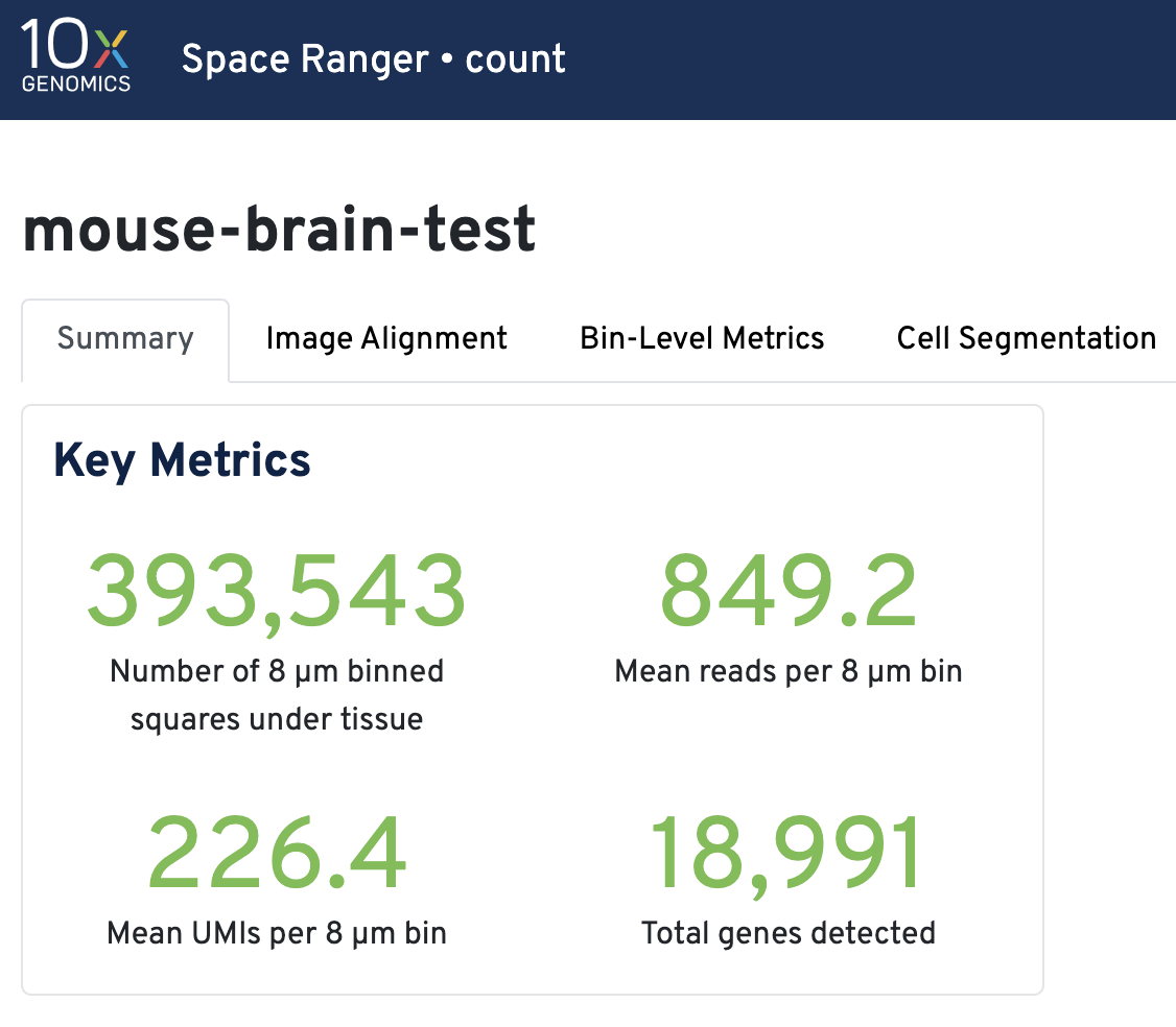
Key metrics include the number of 8 µm binned squares under tissue, mean reads per 8 µm bin, mean UMIs per 8 µm bin, and total genes detected.
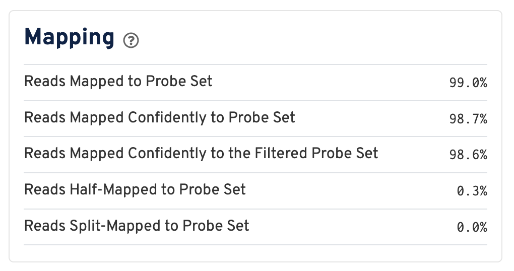
Below the key metrics are the mapping metrics, which will vary depending on whether you are looking at a Visium HD or a Visium HD 3' dataset.
For a Visium HD dataset, reads are mapped to a probe set reference:
Click the ? for definitions:
- Reads Mapped to Probe Set: Fraction of reads that mapped with MAPQ>0 to the probe set.
- Reads Mapped Confidently to Probe Set: Fraction of reads that mapped with MAPQ=255 to one unique probe in the probe set.
- Reads Mapped Confidently to the Filtered Probe Set: Fraction of reads that mapped with MAPQ=255 to one unique probe in the filtered probe set. These reads are considered for UMI counting. See algorithms page for more information on probe filtering.
- Reads Half-Mapped to Probe Set: Fraction of reads that mapped to unpaired ligation products.
- Reads Split-Mapped to Probe Set: Fraction of reads that mapped to mispaired ligation products.
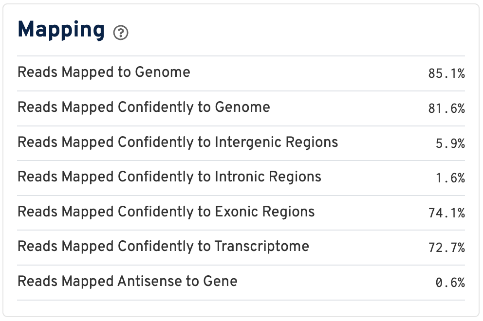
By contrast, for a Visium HD 3' dataset, reads are mapped to a transcriptome reference:
Click the ? for definitions:
- Reads Mapped to Genome: Fraction of reads that mapped to the genome.
- Reads Mapped Confidently to Genome: Fraction of reads that mapped uniquely to the genome. If a gene mapped to exonic loci from a single gene and also to non-exonic loci, it is considered uniquely mapped to one of the exonic loci.
- Reads Mapped Confidently to Intergenic Regions: Fraction of reads that mapped uniquely to an intergenic region of the genome.
- Reads Mapped Confidently to Intronic Regions: Fraction of reads that mapped uniquely to an intronic region of the genome.
- Reads Mapped Confidently to Exonic Regions: Fraction of reads that mapped uniquely to an exonic region of the genome.
- Reads Mapped Confidently to Transcriptome: Fraction of reads that mapped to a unique gene in the transcriptome. The read must be consistent with annotated splice junctions. These reads are considered for UMI counting.
- Reads Mapped Antisense to Gene: Fraction of reads confidently mapped to the transcriptome, but on the opposite strand of their annotated gene. A read is counted as antisense if it has any alignments that are consistent with an exon of a transcript but antisense to it, and has no sense alignments.
Below the mapping metrics are the sequencing metrics.
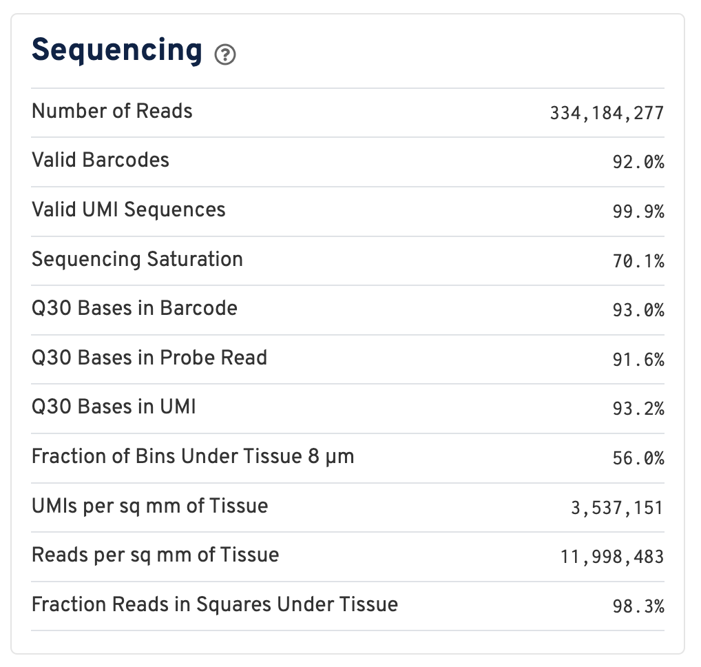
- Number of Reads: Total number of read pairs that were assigned to this library in demultiplexing.
- Valid Barcodes: Fraction of reads with barcodes that match the inclusion list after barcode correction.
- Valid UMIs: Fraction of reads with valid UMIs; i.e. UMI sequences that do not contain Ns and that are not homopolymers.
- Sequencing Saturation: The fraction of reads originating from an already-observed UMI. This is a function of library complexity and sequencing depth. More specifically, this is the fraction of confidently mapped, valid square-barcode, valid UMI reads that had a non-unique square-barcode/UMI/gene combination.
- Q30 Bases in Barcode: Fraction of cell barcode bases with Q-score >= 30, excluding very low quality/no-call (Q < 2) bases from the denominator.
- Q30 Bases in Probe Read: Fraction of RNA read bases with Q-score >= 30, excluding very low quality/no-call (Q < 2) bases from the denominator. This is Read 2 for the Visium v1 chemistry.
- Q30 Bases in UMI: Fraction of UMI bases with Q-score >= 30, excluding very low quality/no-call (Q < 2) bases from the denominator.
- Fraction of Bins Under Tissue 8 µm: Fraction of 8 µm bins covered by tissue.
- UMIs per sq mm of Tissue: Number of UMIs from the Gene Expression library observed per unit area of tissue.
- Reads per sq mm of Tissue: Number of reads from the Gene Expression library observed per unit area of tissue.
- Fraction Reads in Squares Under Tissue: Fraction of valid-barcode, confidently-mapped-to-probe-set reads with tissue-associated barcodes.
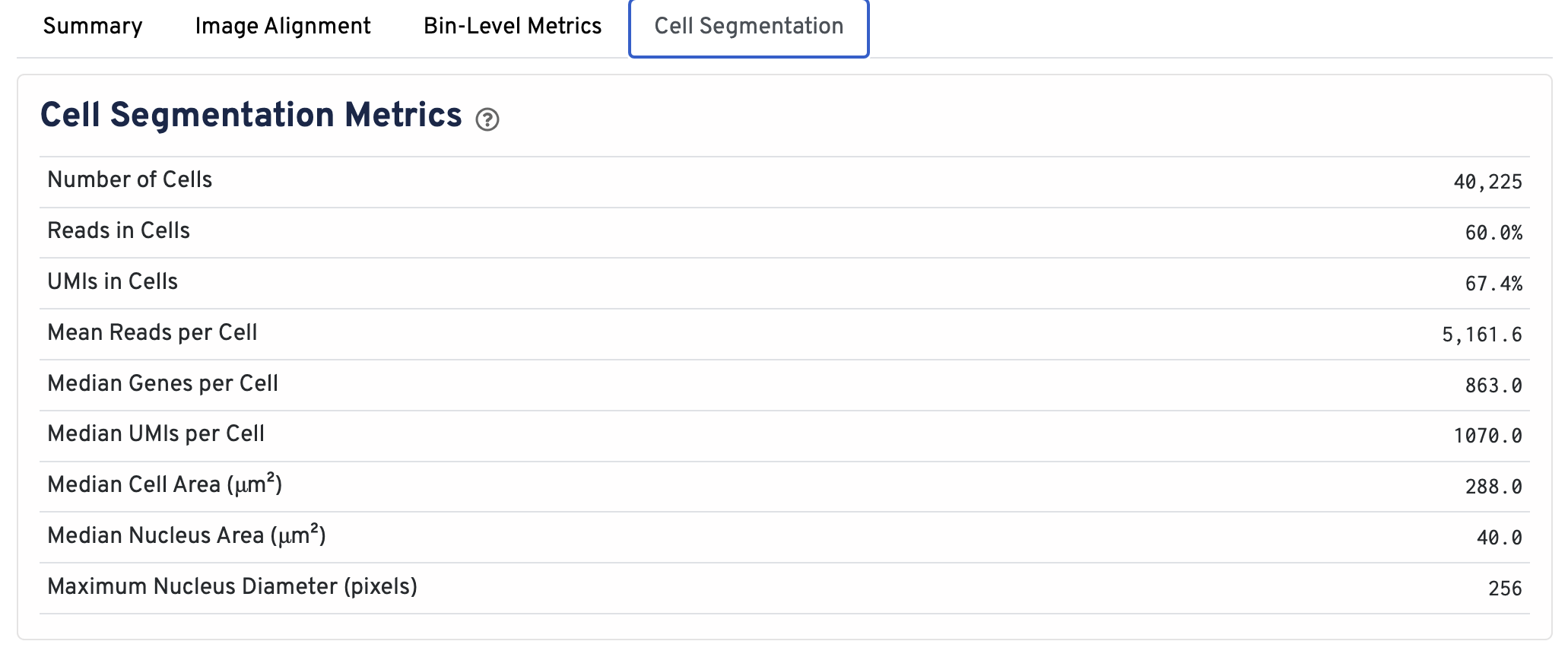
Web summaries output by Space Ranger v4.0 and later include cell segmentation metrics.
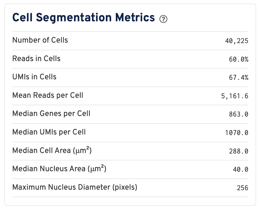
- Number of Cells Detected: The total number of cells with >= 1 unique molecular identifier (UMI).
- Reads in Cells: The total number of reads assigned to cells divided by the total number of reads in the experiment.
- UMIs in Cells: The percentage of UMIs under tissue within cells.
- Mean Reads per Cell: The total number of reads assigned to cells divided by the number of cells.
- Median Genes per Cell: Median number of genes detected per cell. Cells with zero genes detected are excluded from the calculation.
- Median UMIs per Cell: Median number of unique molecular identifiers (UMIs) detected per cell. Cells with zero UMIs are excluded from the calculation
- Median Cell Area (μm²): Each cell area is calculated by the sum area of 2 μm² squares within the segmented cell.
- Median Nucleus Area (μm²): A square is assigned to a nucleus based on the centroid of the square being under the nucleus. Each nucleus area is calculated by the sum area of 2 μm² squares within the segmented nucleus.
- Maximum Nucleus Diameter (pixels): The maximum possible diameter of a nucleus detected in pixels. The segmentation model ensures that nuclei overlapping tile boundaries are detected without being truncated.
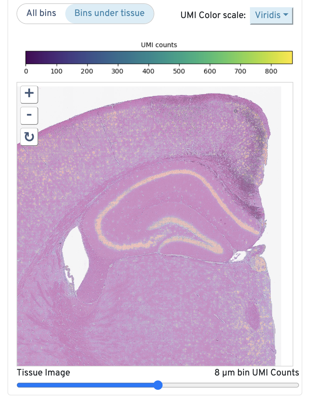
Returning to the top right, observe the Total UMI Count to Image Alignment.
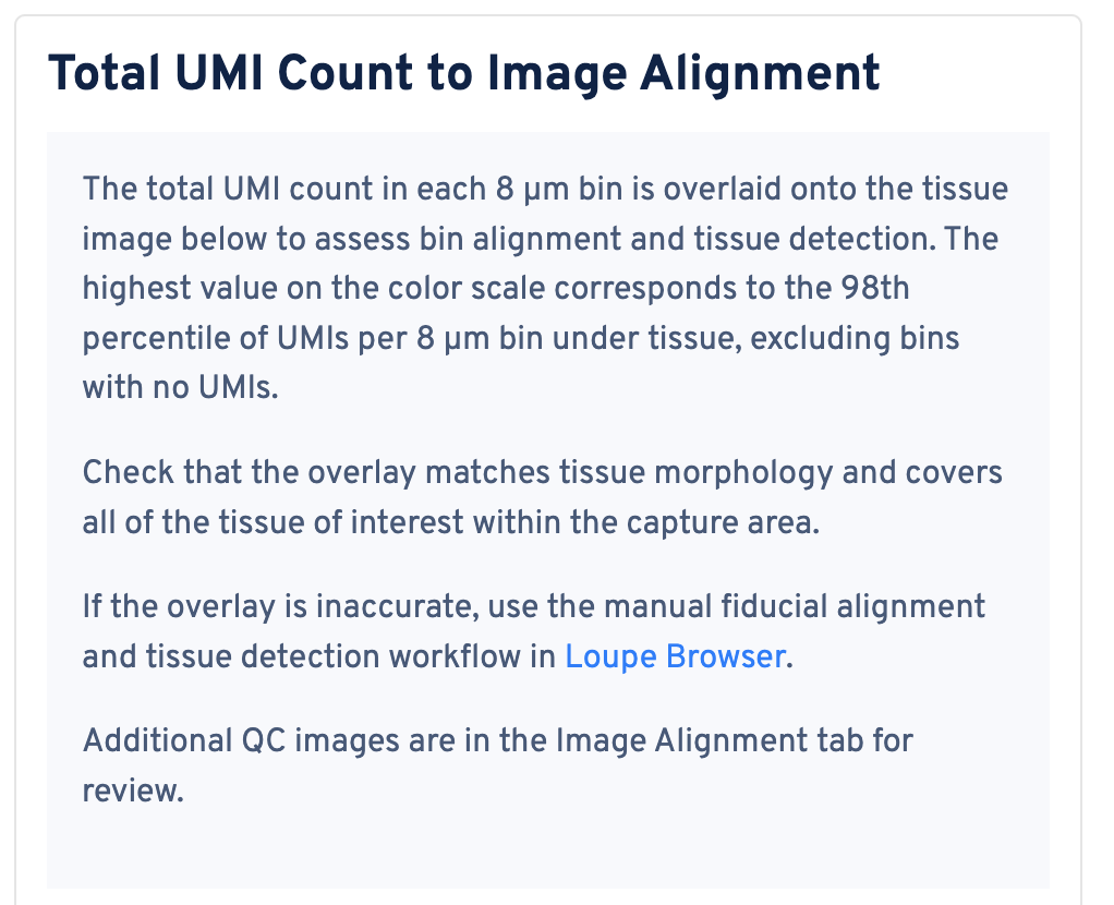
Below the text description, the microscope image is displayed. By default, only bins under tissue are shown, but you can also toggle to view all bins. You can also adjust the color scale and the opacity. Zoom in to check the quality of your alignment.
Below the image are the sample metadata. It is recommended to double check this section for every experiment for any inaccuracies.
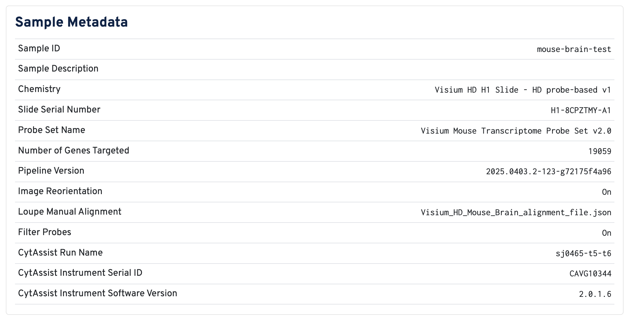
- Sample ID reports the
--idprovided to Space Ranger. - Sample Description displays the optional
--descriptionprovided to Space Ranger, if provided. - Chemistry is inferred from the slide serial number.
- Slide Serial Number includes the capture area as a suffix. This information is provided to the pipeline with the
--slideand--areaoptions and/or the CytAssist image metadata (--cytaimage). For more information about the types of Visium slides compatible with Space Ranger, see the Slide Parameters page. - Probe Set Name indicates which probe set was used (
--probe-set). In this example, the Visium Human Transcriptome Probe Set v2.0 was used. Probe sets are bundled with the Space Ranger pipeline and can also be downloaded from the Download Center. - Number of Genes Targeted means the number of genes targeted by the probeset. This is important to check if you added custom probes to an existing probe set.
- Transcriptome reports which reference was provided to the
--transcriptomeargument. Pre-built references can be retrieved from the Download Center. - Pipeline Version shows the version of Space Ranger that was used to generate the data.
- Image Reorientation is set to true by default, meaning that the pipeline will automatically rotate and/or mirror the microscope image. You can turn it off using
--reorient-images=falseinspaceranger count. - Loupe Manual Alignment will populate with the JSON file, if any, provided to the
--loupe-alignmentoption. - Filter Probes is set to true by default, which is recommended. Otherwise set
--filter-probes=falsewhen runningspaceranger count. - CytAssist Run Name, CytAssist Instrument Serial ID, and CytAssist Instrument Software Version are provided to help with troubleshooting if necessary.
Scroll down to view plots that evaluate sequencing depth.
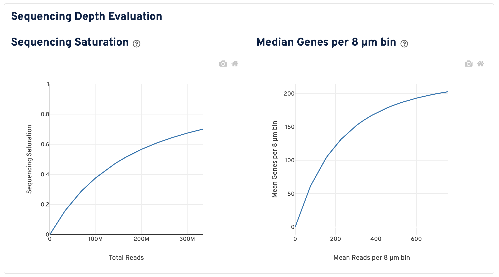
- The Sequencing Saturation plot shows the sequencing saturation metric as a function of downsampled sequencing depth (measured in mean reads per spot), up to the observed sequencing depth. Sequencing Saturation is a measure of the observed library complexity, and approaches 1.0 (100%) when all converted probe ligation products have been sequenced. The slope of the curve near the endpoint can be interpreted as an upper bound to the benefit to be gained from increasing the sequencing depth beyond this point. The dotted line is drawn at a value reasonably approximating the saturation point.
- The Median Genes per 8 µm bin plot shows the mean genes per 8 µm bin as a function of downsampled sequencing depth in mean reads per 8 µm bin, up to the observed sequencing depth. The slope of the curve near the endpoint can be interpreted as an upper bound to the benefit to be gained from increasing the sequencing depth beyond this point.
On the right of this panel is the Segmented Linear Model Plot. Each point represents a gene that has probes targeting both exon-junction-spanning and non-exon-junction-spanning regions, 'spliced' and 'unspliced', respectively. Unspliced probes can stem from open gDNA and from RNA. Spliced probes are expected to stem only from RNA. A segmented linear model is used to estimate where the unspliced and spliced counts begin to deviate. The mean of unspliced counts in purple estimates the UMI background level per unspliced probe. Counts less than this have a high probability of stemming from gDNA.
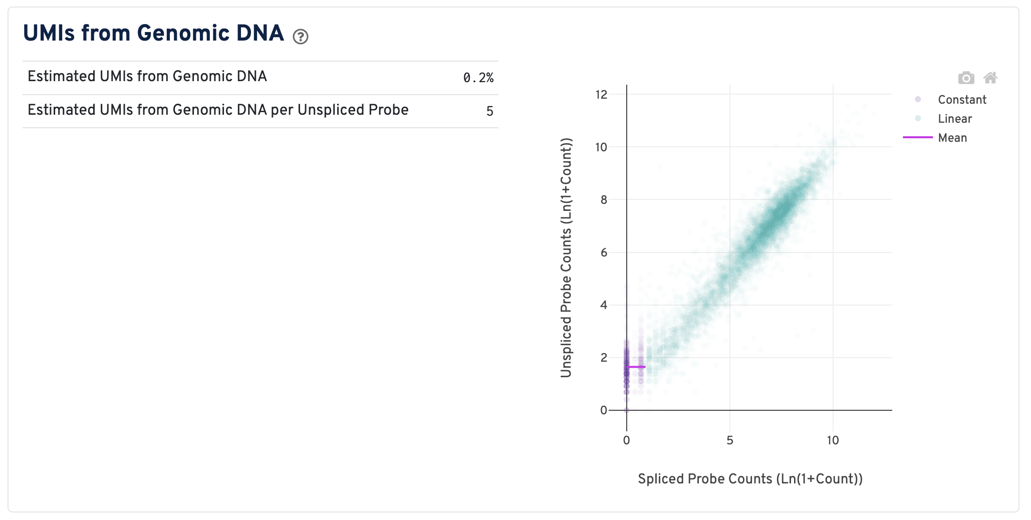
- Estimated UMIs from Genomic DNA: The estimated fraction of filtered UMIs derived from genomic DNA based on the discordance between probes targeting exon-junction-spanning regions and non-exon-junction-spanning regions.
- Estimated UMIs from Genomic DNA per Unspliced Probe: The estimated number of UMIs derived from genomic DNA for each probe targeting non-exon-junction-spanning regions. A probe not spanning an exon junction with a total UMI count below this value has a high likelihood of its UMIs being derived primarily from hybridization to genomic DNA rather than the mRNA. For details, please visit this Tech Note.
On the bottom of this page the exact command line used to run Space Ranger is shown. This can be useful for troubleshooting or record keeping purposes.
Return to the top of the page and click the Image Alignment tab. The Tissue Detection and Fiucial Alignment section is displayed at the top.
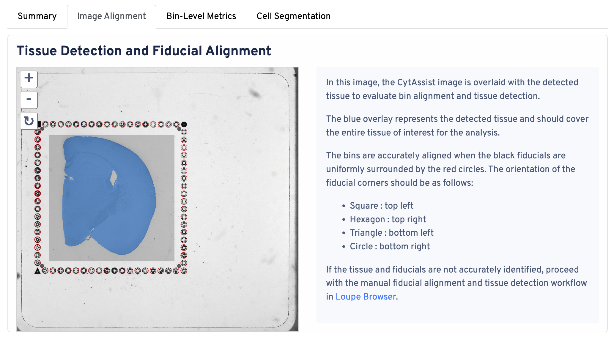
In this image, the CytAssist image is overlaid with the detected tissue to evaluate bin alignment and tissue detection. The blue overlay represents the detected tissue and should cover the entire tissue of interest for the analysis. The bins are accurately aligned when the fiducials are in the correct orientation:
- Square : top left
- Hexagon : top right
- Triangle : bottom left
- Circle : bottom right
If the tissue and fiducials are not accurately identified, proceed with the manual alignment workflow in Loupe Browser.
Next, the CytAssist image and microscope image alignment is shown.

This image shows the registration of the high-resolution microscope image to the CytAssist image. Click and drag the opacity slider between the microscope image and CytAssist image to confirm proper alignment. Zoom in to confirm that tissue boundaries and morphological features are aligned in the two images. If the results indicate poor alignment, use Loupe Browser to perform manual alignment.
This image shows the 8 µm binned total UMI count overlaid on the high-resolution microscope image. If a high-resolution image is not supplied, the CytAssist image is used.
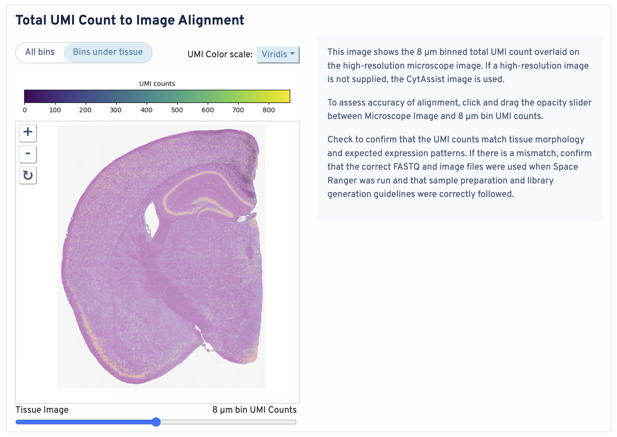
To assess accuracy of alignment, click and drag the opacity slider between Microscope Image and 8 µm bin UMI counts. Check to confirm that the UMI counts match tissue morphology and expected expression patterns. If there is a mismatch, confirm that the correct FASTQ and image files were used when Space Ranger was run and that sample preparation and library generation guidelines were correctly followed.
Return to the top of the page and click the Bin-Level Metrics tab.
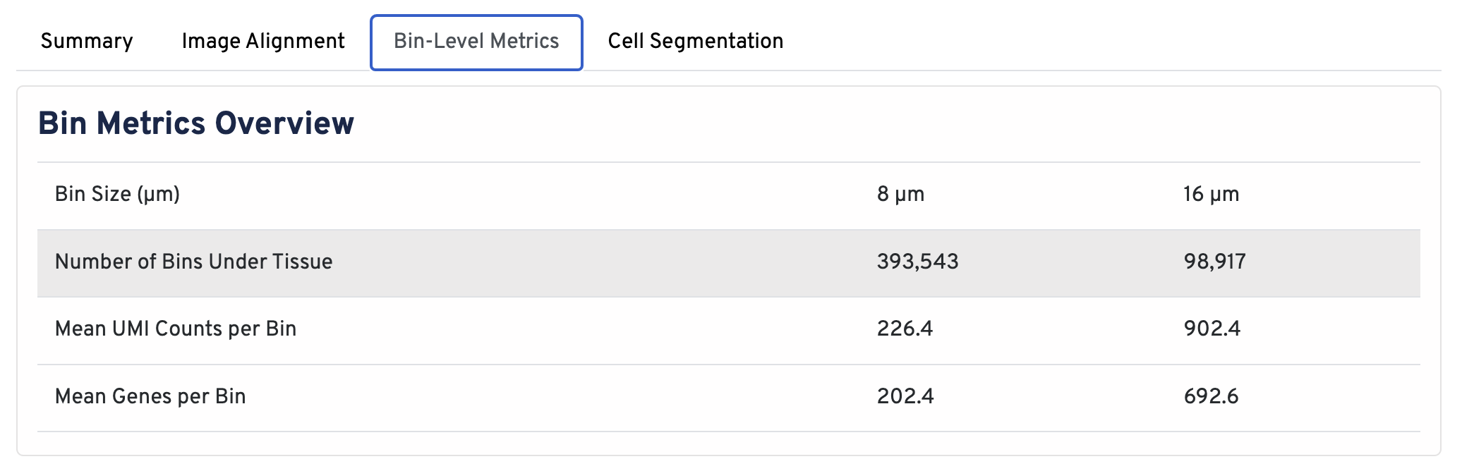
In the Bin Metrics Overview section, metrics are shown for two bin sizes by default, 8 µm and 16 µm.
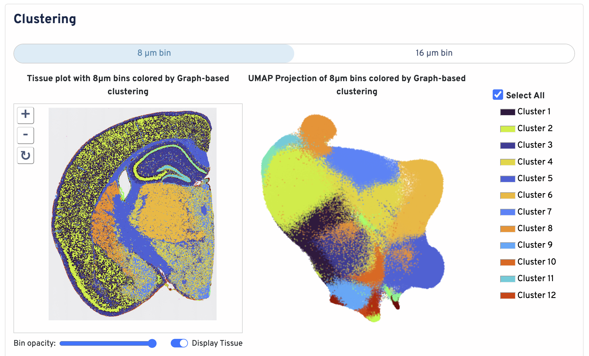
Below the bin metrics are the graph-based clustering plots. You can toggle between the 8 µm and 16 µm bin sizes, hide or display individual clusters, adjust bin opacity, and switch the tissue display.
The differential gene expression (DGE) results are shown in the Top Features by Cluster section below the clustering plots. The differential expression analysis seeks to find, for each cluster, features that are more highly expressed in that cluster relative to the rest of the sample. Here a differential expression test was performed between each cluster and the rest of the sample for each feature.
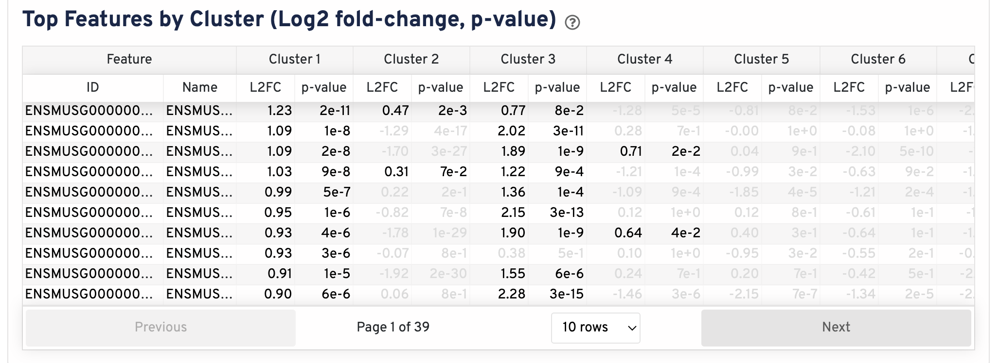
- The Log2 fold-change (L2FC) is an estimate of the log2 ratio of expression in a cluster to that in all other spots. A value of 1.0 indicates 2-fold greater expression in the cluster of interest.
- The p-value is a measure of the statistical significance of the expression difference and is based on a negative binomial test. The p-value reported here has been adjusted for multiple testing via the Benjamini-Hochberg procedure.
In this table, you can click on a column to sort by that value. Also in this table, features were filtered by (Mean UMI counts > 1.0) and the top N features by L2FC for each cluster were retained. Features with L2FC < 0 or adjusted p-value >= 0.10 were grayed out. The number of top features shown per cluster, N, is set to limit the number of table entries shown to 10,000; N=10,000/K^2 where K is the number of clusters. N can range from 1 to 50. For the full table, please refer to the differential_expression.csv files produced by the pipeline, documented on the Secondary Analysis page.
The cell segmentation metrics match those in the Summary tab and are documented earlier on this page.
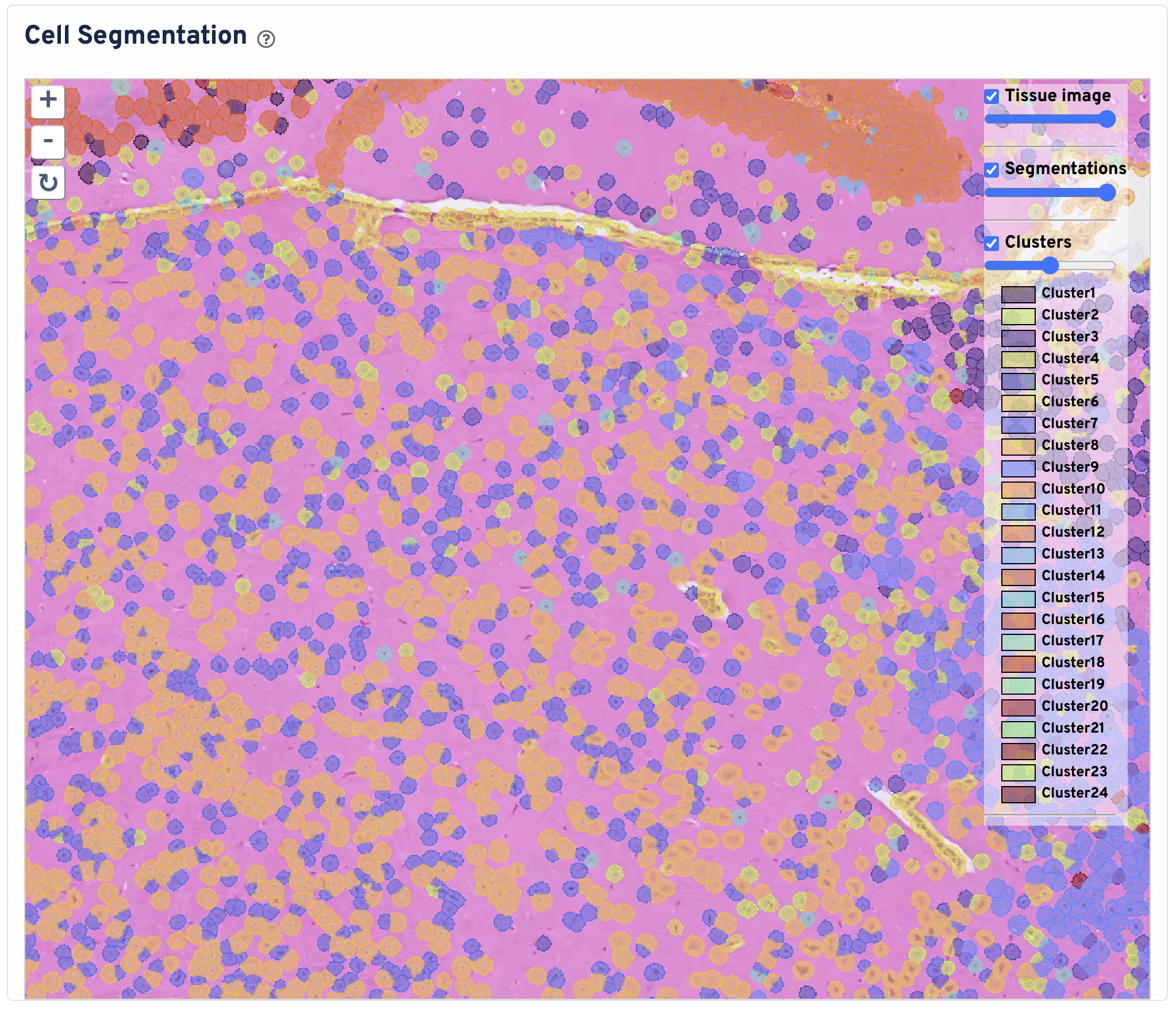
The Cell Segmentation plot shows cells segmented by nucleus expansion. Cell boundaries are colored and filled by graph based clustering assignment. Black box represents the Visium HD capture area. The tissue image is cropped to the capture area + 30 pixels. You can zoom in and out, pan, and toggle the tissue image, segmentations, and clusters. Use this panel to perform initial quality control on your segmentation.
Four additional plots are provided to assess segmentation performance.
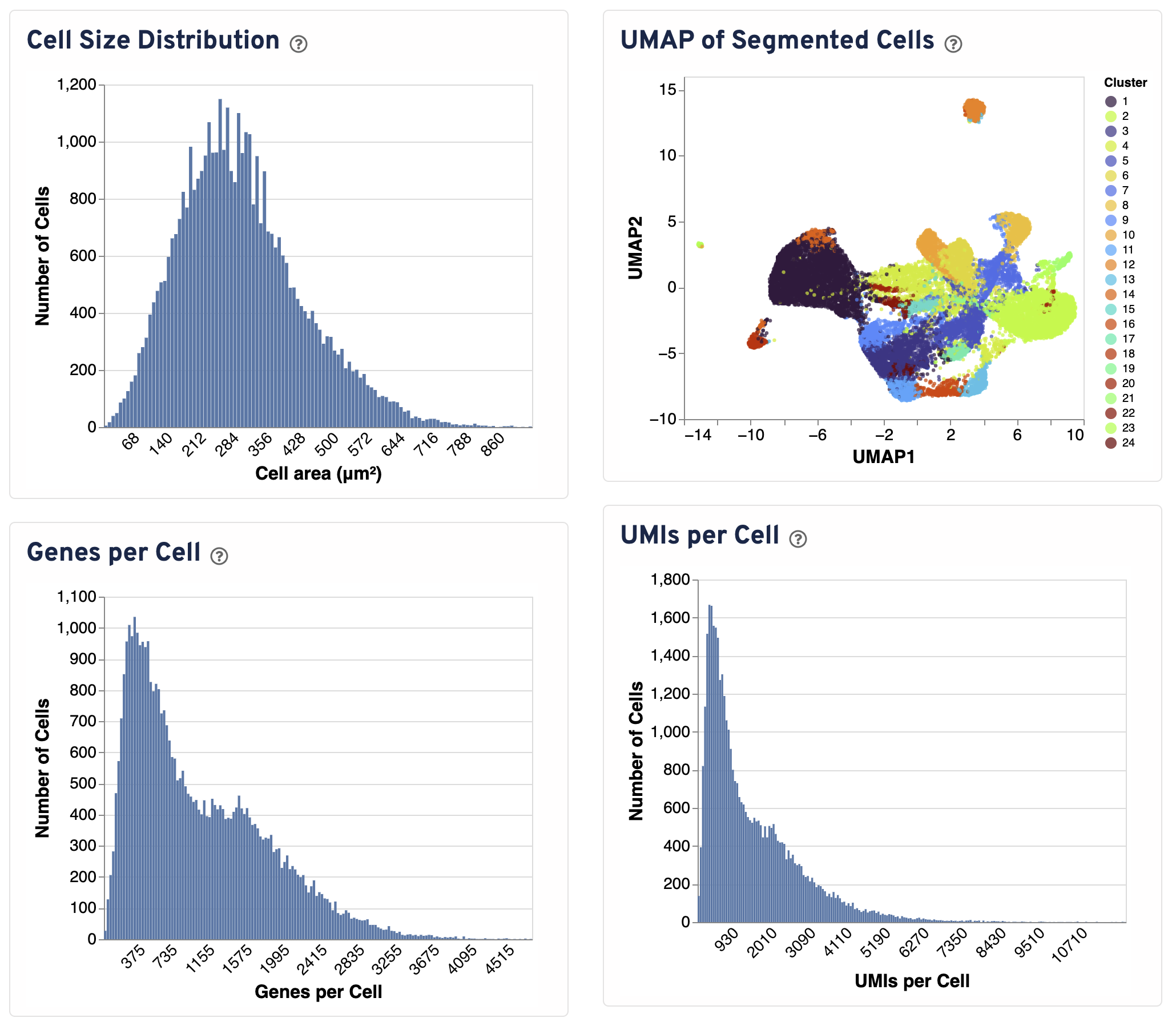
- The Cell Size Distribution plot shows a histogram of areas in μm² for all cells with transcripts. The area is computed from the cell segmentation mask by summing the number of 2 μm² bins.
- The UMAP of Segmented Cells plot is a UMAP representation of segmented cells labeled with graph-based clustering. The plot is sampled to 20,000 cells for visualization purposes.
- The Genes per Cell shows a histogram of the total number of unique genes found in each cell, for all cells with UMIs.
- The UMIs per Cell plot shows a histogram of the total number of UMIs found in each cell over all genes.
The Top Features By Cluster plot shows the differential expression analysis performed downstream of cell segmentation. The differential expression analysis seeks to find, for each cluster, features that are more highly expressed in that cluster relative to the rest of the sample. Here a differential expression test was performed between each cluster and the rest of the sample for each feature.
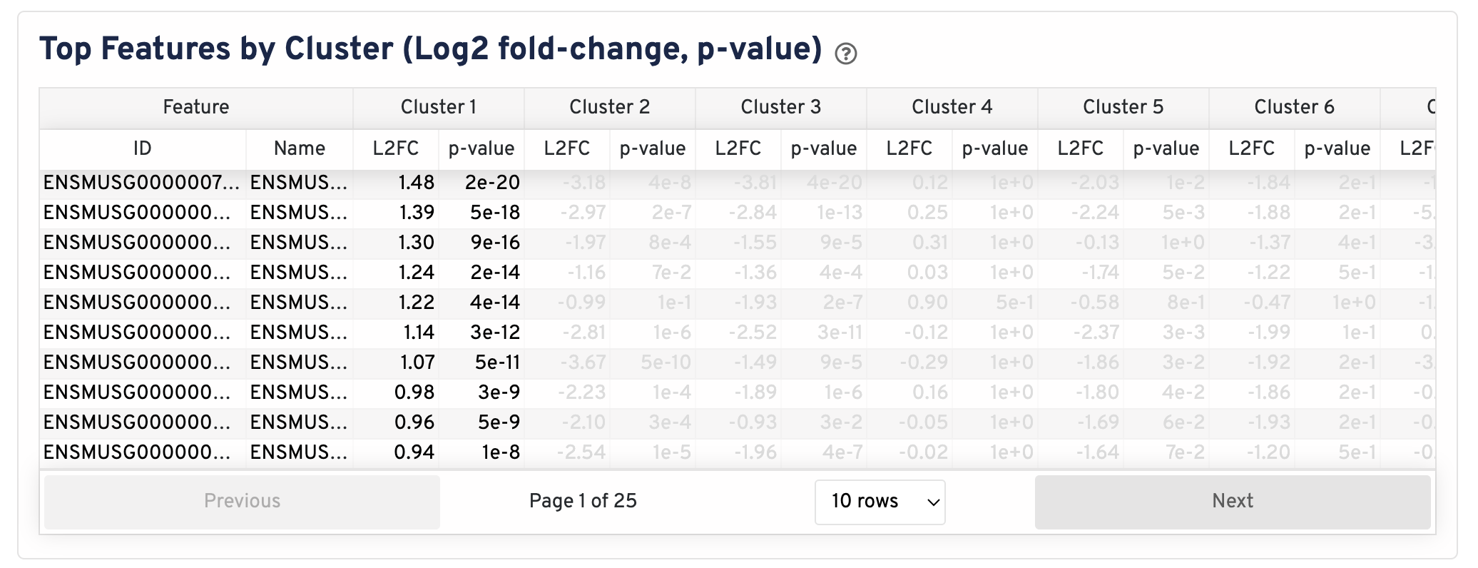
- The Log2 fold-change (L2FC) is an estimate of the log2 ratio of expression in a cluster to that in all other cells. A value of 1.0 indicates 2-fold greater expression in the cluster of interest.
- The p-value is a measure of the statistical significance of the expression difference and is based on a negative binomial test. The p-value reported here has been adjusted for multiple testing via the Benjamini-Hochberg procedure.
In this table, you can click on a column to sort by that value. Also, in this table features were filtered by (Mean object counts > 1.0) and the top N features by L2FC for each cluster were retained. Features with L2FC < 0 or adjusted p-value >= 0.10 were grayed out. The number of top features shown per cluster, N, is set to limit the number of table entries shown to 10,000; N=10,000/K^2 where K is the number of clusters. N can range from 1 to 50. For the full table, please refer to the Secondary Analysis page.