The spaceranger count pipeline outputs several CSV files and dendrogram plots which contain automated LDA-based spot deconvolution results for many values of K topics. The algorithm starts by performing LDA with an initial K = N graph-based clusters + 2 to model the Visium spot data as a mixture of K topics (inferred cell types). It then hierarchically clusters topics and collapses branches for decrementing K until K =2. See the algorithms page for more details.
The results are organized in the deconvolution folder as follows.
| File Name | Description |
|---|---|
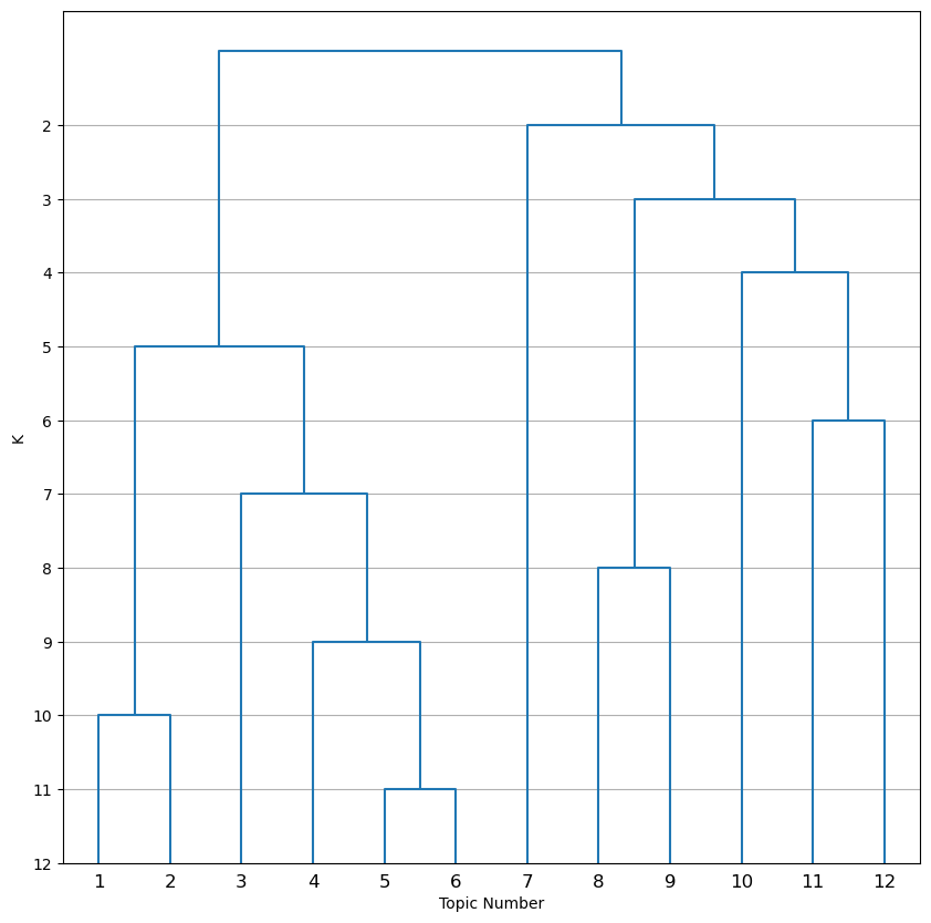
| deconvolution/dendrogram_k.png | Dendrogram showing how topics are hierarchically clustered and collapsed down to K = 2 |
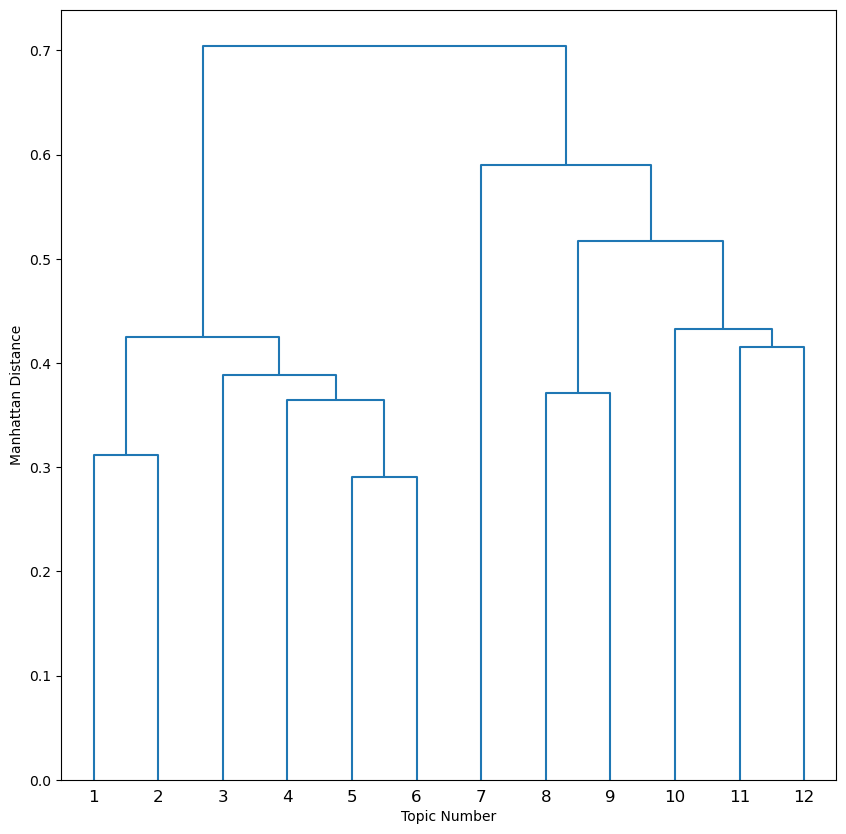
| deconvolution/dendrogram_k_distances.png | Dendrogram showing how topics are hierarchically clustered by distance between topics |
| deconvolution/deconvolution_k/ | Folders containing deconvolution results for every K |
| deconvolution/deconvolution_k/deconvolution_topic_features_k.csv | Contains pseudocount and log2 fold change of features in each topic for annotating topics with cell type |
| deconvolution/deconvolution_k/deconvolution_spots_k.csv | Contains the estimated proportions of each topic within every spot |
For a dataset with 10 graph-based clusters (largest K = 12), the deconvolution_topic_features_k12.csv is a table of topics and features that shows the relevance of every feature to each topic. It can be used for annotating topics to their biological cell type.
The column headers are: Feature ID, Feature Name, Feature count topic 1, Feature log2 fold change topic 1, Feature count topic 2, Feature log2 fold change topic 2, …
The feature count for each topic is a pseudocount of the number of UMIs assigned to each topic after LDA over the entire tissue. The log2 fold change calculates the increase of the feature in that topic relative to all other topics and quantifies the relevance of the gene to a topic.
The deconvolution_topic_features CSV for smaller K’s have topics named to indicate which topics were collapsed together. For example topic 1to2 is a topic that combines topic 1 and topic 2 together from the highest level of K.
The deconvolution_spots_k12.csv is a table of topics and spot barcodes that show the proportion of topics found in each spot under tissue. The sum of topic proportions for each spot is always equal to 1.
The column headers are: Barcode, Topic 1, Topic 2, …
The deconvolution_spots CSV for smaller K values have topics named to indicate which topics were collapsed together. For example topic 1to2 is a topic that combines topic 1 and topic 2 together from the highest level of K.
The dendrogram_k12.png shows the order of branching. X axis has the topics for largest initial K and the Y axis shows where the branches are cut for every level of K. For example, at K = 10, Topics 1 and 2 are collapsed to Topic 1to2 and Topics 5 and 6 are collapsed to Topic 5to6.
The dendrogram_k12_distances.png uses height to convey similarity of topics in addition to the order of branching. For example, in this plot it is apparent that topics 10, 11, and 12 are almost equally similar to each other even though from the other dendrogram it may seem like topics 11 and 12 are much more similar to each other than to topic 10.